Short Premium Research Dissection (Part 37)
Posted by Mark on June 27, 2019 at 07:02 | Last modified: January 8, 2019 05:53In this “most up-to-date” section (see end Part 31), our author has explored time stops, delta stops, and now profit targets.
As a prelude to determine what profit targets are suitable for backtesting, she gives us this table:
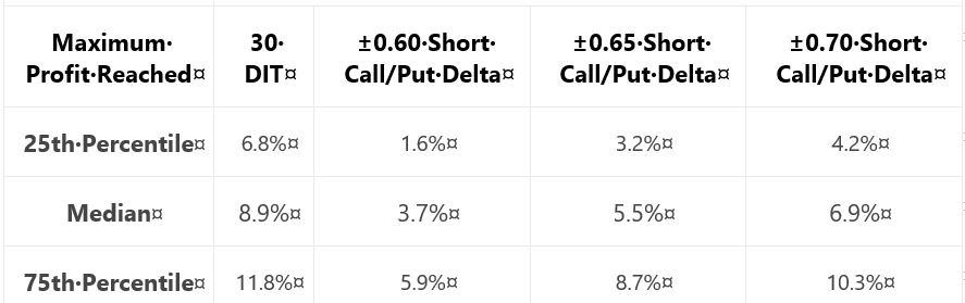
Recall from the end of Part 35 that when something changes without explanation, the critical analyst should ask why. She did not include the 0.65-delta stop last time: why? In this case, it’s no big deal. I like backtesting over a parameter range and having three values across the range is better than two. If only for the sake of consistency, I would have liked to see 0.65 data both times because it feels sloppy when things change from one sub-section to the next.
Adding to the sloppiness, she is once again lacking in methodology detail. I like the idea of probing the distribution to better understand where profit might land. If we can’t replicate, though, then it didn’t happen. Did she backtest:
- Daily trades?
- Non-overlapping trades?
- Winners?
- Winners and losers?
- Any [combinations] of the above?
These factors can all shape our expectations for sample size (which determines how robust the findings may be) and magnitude of averages (e.g. winners will have a higher average max profit than winners and losers. See Part 24 calculations).
She writes:
> Based on the above table, it appears profit targets
> between 5-10% seem reasonable to test for all of the
> approaches except the ±0.60 delta-based trade exits.
She then proceeds to give us “hypothetical portfolio growth” graph #17 with [hypothetical computer simulated performance disclaimer and] 30 DIT, 5% profit target or 30 DIT, and 10% profit target or 30 DIT.
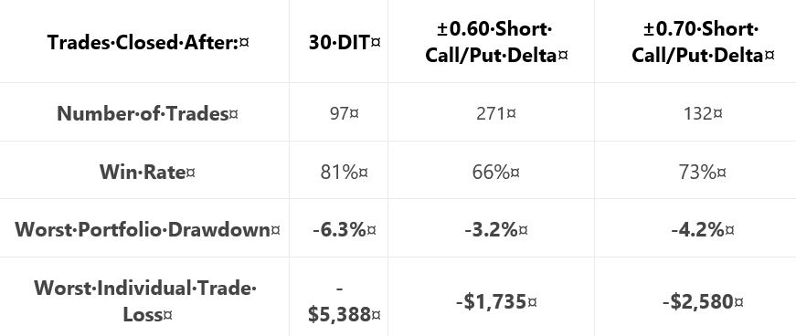
Next, she gives us a “hypothetical portfolio growth” graph and table each for 0.65- and 0.70-delta stops. The graphs are all similar with no allocation, no inferential statistics, and nebulous profitability differences. The tables take the following format:
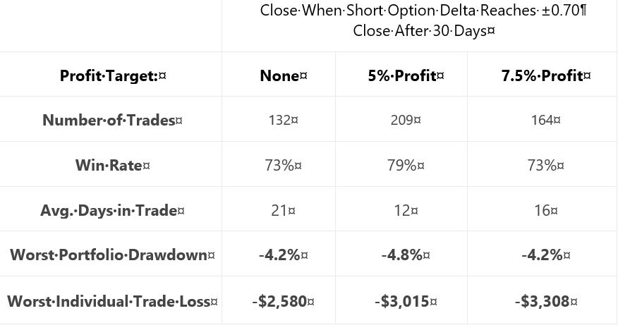
This falls far short of the standard battery and also lacks a complement of daily trade backtesting (see fourth-to-last paragraph here). We still don’t know her criteria for adopting trade guidelines, either. I therefore like her [non-]conclusion:
> After analyzing the various approaches and management
> levels, it seems you could pick any one of the variations
> and run with it. Consistency seems to be more important
> than the specific numbers used to trigger your exits.
She also writes:
> Interestingly, not using a profit target with the ±0.70
> delta-based exit was the ‘optimal’ approach historically.
For this reason and because she did not test [all permutations of] each condition[s], I remain uncertain whether a delta stop is better than any or no time stop. I would say the same about profit target: too much sloppiness and too few methodological details [and transaction fees as discussed at the end of Part 36] to know whether it should make the final cut.
I will continue next time.
Categories: System Development | Comments (0) | PermalinkShort Premium Research Dissection (Part 36)
Posted by Mark on June 24, 2019 at 07:10 | Last modified: January 2, 2019 11:17Picking up right where we left off, our author gives the following [partial] methodology for her next study:
> Expiration: standard monthly cycle closest to 60 (no less than 50) DTE
> Entry: day after previous trade closed
> Sizing: one contract
> Management 1: Hold to expiration
> Management 2: Exit after 30 days in trade (10 DIT)
I think this should be “30 DIT.” The proofreader fell asleep (like third-to-last paragraph here).
Here is “hypothetical portfolio growth graph” #15:
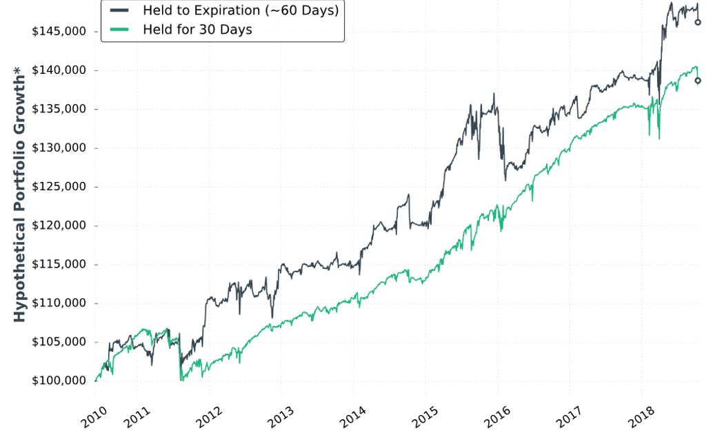
The two curves look different; a [inferential] statistical test would be necessary to quantify this.
She concludes the time stop results in smoother performance and smaller drawdowns. Once again, I’d like this quantified (e.g. the standard battery). I’d also like a backtest of daily trades (rather than non-overlapping) for more robust statistics.
Next, she adds delta stops:
> Management 1: Hold for 30 days (30 DIT)
> Management 2: Exit when short call delta hits +0.60 OR the short put delta hits -0.60
> Management 3: Exit when short call delta hits +0.70 OR the short put delta hits -0.70
I like the idea of a downside stop, but I question the upside stop. With an embedded PCS, we are already protected from heavy upside losses. She does not test downside stop only.
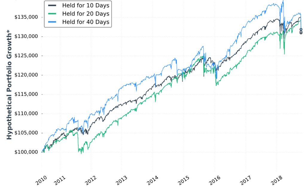
Here is “hypothetical portfolio growth” graph #16:
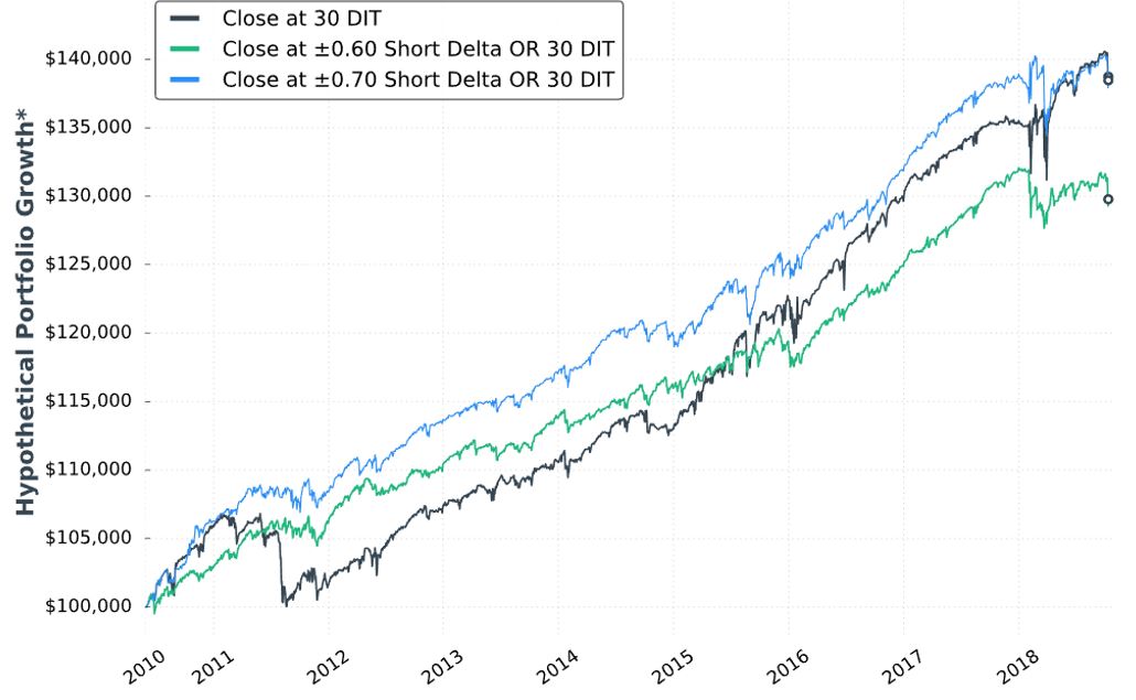
The blue curve finishes at the top and is ahead throughout. The black curve finishes on top of the green, but only leads the green for roughly half the time. Inferential statistics would help to identify real differences.
Thankfully, each of the last two graphs are presented with that “hypothetical computer simulated performance” disclaimer (see second paragraph below graph in Part 34).
Here are selected statistics for graph #16:
As discussed in the second-to-last paragraph here, percentages are not useful on a graph without allocation. I think relative percentages can be compared, however, when derived on the same allocation-less backdrop.
Unfortunately, we have no context with which to compare total return. As mentioned above, we’re lacking the standard battery (second paragraph) and complement of statistics for daily trades.
As with Part 34, other glaring table omissions include average DIT (to understand impact of delta stops), and PnL per day.
Transaction fees (TF) could adversely affect the delta-stop groups because they include more trades. Our author now mentions fees for the first time:
> …many more trades are made… [with] delta-based exit… we need to
> be considerate of commissions… [At] $1/contract, the ±0.60 delta exit
> would… [generate] $2,168 commissions… if you trade with tastyworks,
> the commission-impact of the strategy could be substantially less…
Unfortunately, she mentions fees only to give a brokerage commercial. Her affiliation with the brokerage is clear because she offers the research report free if you open an account with them. In and of itself, this conflict of interest would constitute a fatal flaw for some.
Discussing commissions but not slippage is sloppy and suspect. It is sloppy because as a percentage of total TF, slippage is much larger than commissions. It is suspect because neither is factored into the backtesting, which makes results look deceptively good.
Thus ends another sub-section with nothing definitive accomplished. She may or may not include time- or delta-based stops in the final system and if she does, then she has once again failed to provide any conclusive backing for either (also see third paragraph below first excerpt here).
Categories: System Development | Comments (0) | PermalinkShort Premium Research Dissection (Part 35)
Posted by Mark on June 21, 2019 at 07:37 | Last modified: January 3, 2019 06:54Finishing up the sub-section from Part 34, our author writes:
> At the very least, when incorporating short premium options
> strategies… it may be wise to implement time-based exits
> to avoid large/complete losses and reduce portfolio volatility.
By not stating definitive criteria, she [again] tells us nothing conclusive. As discussed in the second paragraph after the first excerpt here, we’ll have to wait to see if a time stop makes the final cut.
Unlike the 50% profit trigger for rolling puts to 16 delta, I think the time stop is beneficial. I wish she had shown us the top 3 drawdowns as done previously (e.g. Part 31 table). Seeing improvement on each of the top 3 would be stronger support for time stops than improvement on just the worst. Even better would be the entire standard battery (second paragraph).
Unfortunately, we do not know how time stops would impact the high-risk strategy, which was backtested before 2018.
I can’t help but wonder why time stops were not studied before 2018 (final excerpt Part 31). Admittedly, I would have suspected curve fitting had she written “due to the horrific drawdown suffered in Feb 2018, I tried to add some conditions to make the strategy more sustainable.” Not giving any explanation makes me suspect the same. I think the best approach to avoid being influenced by disappointing results is to plan the complete research strategy in advance (second paragraph below excerpt here). Exploring the surrounding parameter space (see second paragraph here) is critical as well.
> The next trade management tactic we’re going to explore
> is the idea of ‘delta-based’ exits.
Like time stops, this is another completely new idea for her. As just discussed, this ad hoc style bolsters my suspicion (see third paragraph below excerpt in Part 30) that she spontaneously tosses out ideas with the hope of finding one that works. Given enough tests, success by chance alone is inevitable. “Making it up as we go along” to cover for inadequate performance is a flawed approach to system development.
> To verify the validity of using delta-based exits, let’s look
> at some backtests to compare holding to expiration, adding
> a time-based exit, and then adding a delta-based exit.
Layering conditions is confusing because order may matter* and all permutations are not explored (see second and third paragraphs here). For example, she does not study a delta-based exit without a time-based exit. I would rather see each condition tested independently with those meeting a predetermined performance requirement making the final cut.
> First, let’s compare… holding to expiration… [with]…
> exiting after 30 DIT.
Where did 30 come from? The exploratory studies (Part 34) looked at 10, 20, and 40 DIT.
When something changes without explanation, the critical analyst should ask why. This is becoming a recurring theme (as mentioned hear the end of Parts 32 and 33).
I will continue next time.
* In statistics, this is called interaction.
Short Premium Research Dissection (Part 34)
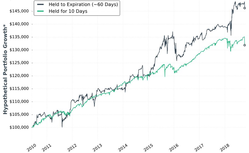
Posted by Mark on June 18, 2019 at 07:00 | Last modified: December 31, 2018 13:29Continuing with exploration of time stops, our author gives us hypothetical portfolio growth graph #15:
As discussed last time, this is based on one contract traded throughout. The hypothetical portfolio is set to begin with $100,000. This is fixed-contract position sizing. One consequence of fixed-contract versus fixed-risk (fractional) is a more linear equity curve rather than exponential. As discussed [here], the latter reaches higher and looks more appealing despite having greater risk. I have traditionally been a proponent of omitting position sizing from backtesting to allow for what I thought would be apples-to-apples comparison of drawdowns throughout (see here). In these graphs without any allocation, position sizing is effectively eliminated from the equation.
Accompanying the graph is that disclaimer about hypothetical computer simulated performance. This was a big deal earlier in the mini-series when I discussed the asterisk following the y-axis title “hypothetical portfolio growth” (second paragraph here). The disclaimer appeared for the first time in Part 16 and alleviated many pages of confusion. After that, the disclaimer disappeared leaving the asterisk without a referent until the two most recent graphs.
Score a point for completeness—however transient it may be—rather than footnote false alarm and sloppiness.
I can’t discern much with regard to differences on this graph. Final equity is ~$130,000 for all. 40 DIT > 10 DTE > 20 DTE for most of the backtesting interval, which suggests these differences might be significant were inferential statistics to be run.
She gives us the following table:
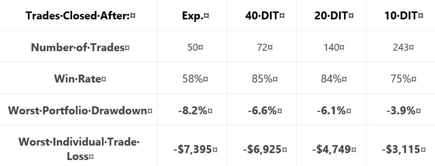
This is not the first time she tells us number of trades, but she falls far short of reporting it every time. Number of trades range from 50 – 243 over roughly eight years. That is ~6 – 30 trades per year or ~0.5 – 2.5 trades per month. On their own, these aren’t tiny samples. Backtesting one starting every trading day (e.g. second paragraph below graph here), though, would give a sample size in the thousands. I think that would be a useful complement to what we have here.
Glaring omissions in this table include average DIT (for the expiration group), total return or CAGR, and PnL per day. A big reason for using a time stop is to improve profitability (either gross or per day): show us! Time stops aim to exit trades earlier: show us [how long they run otherwise]! Nothing is conclusive without these.
Another big shortfall is the exclusion of transaction fees. Number of trades varies 2-5x across groups. The fees could add up.
I would still like to see that lost data [discussed last time] back to 2007.
On the positive side, the table does a decent job of showing performance improvement with max DD and max loss if we assume equal total return as suggested in the graph.
Categories: System Development | Comments (0) | PermalinkShort Premium Research Dissection (Part 33)
Posted by Mark on June 13, 2019 at 07:07 | Last modified: December 29, 2018 06:31I continue today with the second-to-last paragraph on allocation.
All graphs from previous sections assume allocation. Some graphs study allocation explicitly (e.g. Part 20). Others incorporate a set allocation to study different variables (e.g. 5% in Part 18). Return and drawdown (DD) percentages may be calculated from any of these allocation-based graphs.
I remain a bit uneasy about the fact that so many of the [estimated] CAGRs seen throughout this report seem mediocre (see fifth paragraph here). I am familiar with CAGR as it relates to long stock, which is why I have mentioned inclusion of a control group at times (e.g. paragraph below graph here and third paragraph following table here).
While [estimated] CAGR has me concerned, CAGR/MDD would be a more comprehensive measure (see third-to-last paragraph here). Unfortunately, I am not familiar with comparative (control) ranges for CAGR/MDD on underlying indices, stocks, or other trading systems. Unlike Sharpe ratio and profit factor—metrics with which I am familiar regardless of market or time frame—I rarely see CAGR/MDD discussed.
The larger takeaway may be as a prerequisite to do or review system development. I would be more qualified to evaluate this research report were I to have the intuitive feel for CAGR/MDD that I have for Sharpe ratio and profit factor.*
With regard to the Part 32 graph, our author writes:
> The two management approaches were profitable… Holding trades
> to expiration was an extremely volatile approach, while closing
> trades after 10 days… resulted in a much smoother ride.
That [green] curve looks smoother, but volatility of returns cannot be precisely determined especially when four curves are plotted on the same graph. This is a reason I promote the standard battery (see second paragraph of Part 19): standard deviation of returns and CAGR/MDD are the numbers I seek. Inferential statistics would also be useful to determine whether what appears different in the graph is actually different [based on sample size, average, and variance].
Now back to the teaser that closed out Part 32: did you notice something different between that graph and previous ones?
For some unknown reason, we lost three years of data: 2007-2018 in previous graphs versus 2010-2018 in the last.
This “lost data” is problematic for a few different reasons. First, 2008-9 included the largest market correction in many years. Any potential strategy should be run through the period many people consider as bad as it gets especially when the data is so easily available. Second, inclusion of system guidelines thus far has been made based on largest DDs and/or highest volatility levels: both of which included 2008 [this isn’t WFA]. Finally, when something changes without explanation, the critical analyst should ask why. Omitting 2008 from the data set could be a great way to make backtested performance look better. This would be a curve-fitting no-no, which is why it raises red flags.
* This is a “self-induced shortcoming,” though. Any mention of CAGR/MDD in this mini-series comes
from my own calculation (e.g. second paragraph below table in Part 20). Our author makes no
mention of these while omitting many others as well.
Short Premium Research Dissection (Part 32)
Posted by Mark on June 10, 2019 at 06:41 | Last modified: December 31, 2018 15:07Early in Section 5, our author recaps:
> In the previous section, we… constructed with a 16-delta long put…
> and long 25-delta call.
>
> The management was quite passive, as trades were only closed
> when 75% of the maximum profit… or expiration was reached.
We now know the rolling was not adopted after all (see second paragraph below first excerpt here).
> …achieving 75% of the maximum profit potential is unlikely… we
> are holding many trades to expiration, or very close to expiration.
> That’s because if the stock price is… [ATM]… most of the option
> decay doesn’t occur until the final 1-2 weeks before expiration.
I addressed this in the last paragraph here.
> On average, trades were held for 50-60 days, which means few
> occurrences were traded each year and the performance of those
> trades sometimes swung wildly near expiration.
We finally get an idea about DIT (part of my standard battery as described in this second paragraph). She also admits use of a small sample size, which backs my concern about a couple trades drastically altering results (e.g. third-to-last paragraph of Part 29). In the paragraph below the first excerpt of Part 31, I talked about that high PnL volatility of the final days.
> To solve the issue of volatile P/L fluctuations when holding…
> near expiration, we can… [close] trades… after a certain
> number of calendar days in the trade. I’ll refer to this as
> Days In Trade (DIT).
Yay time stops! I suggested this in that last paragraph of Part 25.
For the first backtest of time stops, she gives us partial methodology:
> Expiration: standard monthly cycle closest to 60 (no less than 50) DTE
In other words, trades are taken 50-80 DTE. I would like to see a histogram distribution of DTE since these are not daily trades (see Part 19, paragraph #3).
> Entry: day after previous trade closed
> Sizing: one contract
Number of contracts is new. This makes me realize she changed from backtesting the ETF to the index. It shouldn’t matter one way or another, but when something changes without explanation, the critical analyst should ask why.
> Management 1: hold to expiration
> Management 2: exit after 10 DIT
She gives us hypothetical portfolio growth graph #14:
She writes:
> Note: Please ignore the dollar returns in these simulations.
> Pay attention to the general strategy performance. The last
I have wondered about how to interpret these graphs since the second one was presented at the end of Part 7.
> piece we’ll discuss is sizing the positions and we’ll look at
> historical strategy results with various portfolio allocations.
This suggests the graph is done without regard to allocation. With the strategy sized for one contract, I’m guessing the y-axis numbers to be arbitrary yet sufficient to fit the PnL variation. This also means I cannot get meaningful percentages from the graph. As an example, the initial value could be $100,000,000 or $100,000 and still show all relevant information. The percentages would differ 1000-fold, however.
I will now leave you with the following question: as seen above, what unexplained change was made to the graph format that frustrates me most?
Categories: System Development | Comments (0) | PermalinkShort Premium Research Dissection (Part 31)
Posted by Mark on June 7, 2019 at 06:55 | Last modified: December 27, 2018 06:30Our author concludes Section 4 with a study of different profit targets. She briefly restates the incomplete methodology and gives us hypothetical portfolio growth graph #13:
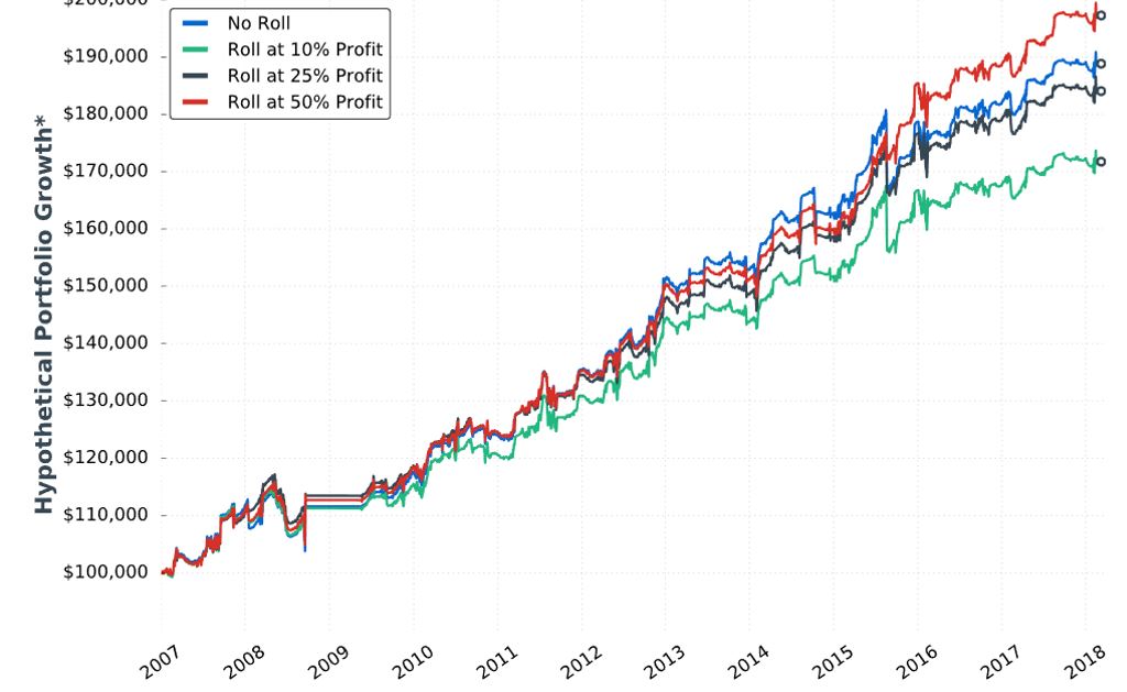
She gives us the following table:
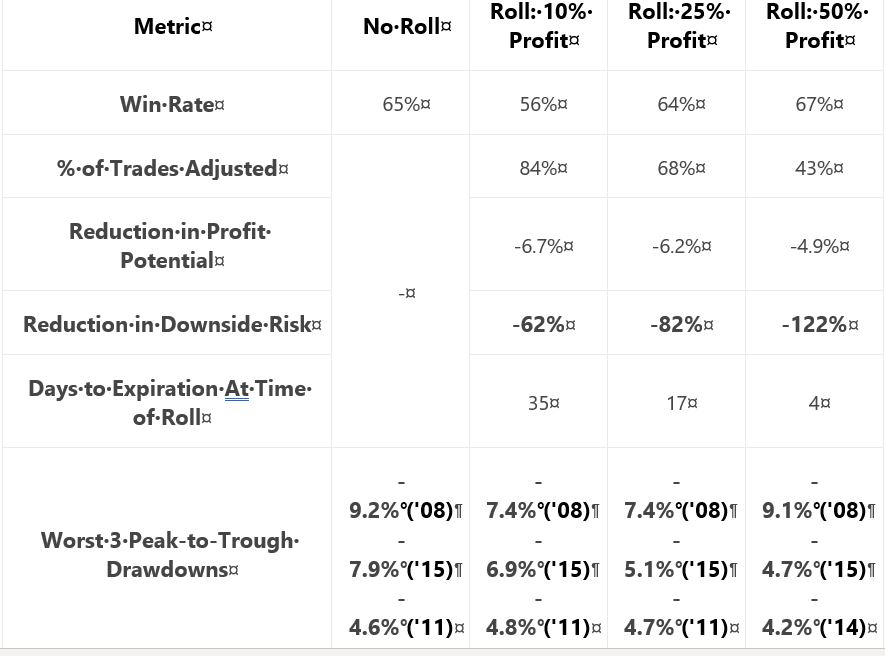
My critiques should be familiar:
- No sample size given
- No inferential statistics provided
- CAGR not given to reveal profitability
- Uncertain DD improvement with four of 18 comparison results unexpected (see second paragraph below table here)
She writes:
> …the downside of waiting until 50% profits is that… long put
> adjustment might not be made at all (which was the case 57%
> of the time), which means the trade’s risk was not reduced. This
> explains why the 50% profit… trigger suffered a very similar
> drawdown compared to… no trade adjustments.
My comments near the end of Part 27 once again apply. This adjustment helps only in case of whipsaw. With the 50% profit trigger, that whipsaw would have to occur inside 4 DTE. If I’m going to bet on extreme PnL volatility, then I would bet on the final four days. However, based on my experience the higher probability choice would be to simply exit at 4 DTE.
I don’t think rolling the put to 16-delta should be part of the final trading strategy. Doing so looks to underperform as shown in the Part 27 graph. If rolling is adopted then, in looking at the above graph, is there any way a 50% profit target adjustment trigger (as opposed to 25%) should not be adopted as well? This would be something to revisit after Section 5 when the completely trading strategy is disclosed.
Criteria for acceptable trading system guidelines should be determined before the backtesting begins as discussed in the second paragraph below the excerpt here. By defining performance measures (also known as the subjective function) up-front, whether to adopt a trade guideline should be clear.
Let’s move ahead to the final section of the report. Our author writes:
> In late 2018, I dove back into the research to analyze
> trade management rules that would accomplish two goals:
>
> 1) Reduced P/L volatility (smoother portfolio growth curve)
> 2) Limit drawdown potential
These should be goals of any trading strategy. Certainly #2 was a focus before because she has talked about top 3 drawdowns throughout the report. I have spent much time discussing it.
I have been clamoring to see standard deviation (SD) of returns as part of the standard battery (see second paragraph here) throughout this mini-series. SD would be a measure for #1.
> In this section, you’re going to learn my most up-to-date
> trading rules and see the exact strategy I use…
What I do not want to see are additional rules added only to make 2018 look better. That would be curve fitting.
I will go forward with renewed optimism and anticipation.
Categories: System Development | Comments (0) | PermalinkShort Premium Research Dissection (Part 30)
Posted by Mark on June 4, 2019 at 06:40 | Last modified: December 26, 2018 06:36I left off feeling like our author was haphazardly tossing out ideas and cobbling together statistics to present whatever first impressions were coming to mind.
The whole sub-section reminds me of something I read from Mark Hulbert in an interview for the August 2018 AAII Journal:
> …people’s well-honed instincts, which detect outrageous
> advertising in almost every other aspect of life, somehow
> get suspended when it comes to money. If a used car salesman
> came up to somebody and said, “Here’s a car that’s only been
> driven to church on Sundays by a grandmother,” you’d laugh.
> The functional equivalent of that is being told that all the
> time in the investment arena, and [responding] “Where do I
> sign up?” The prospect of making money is so alluring that
> investors are willing to suspend all… rational faculties.
As discussed in this second-to-last paragraph, I miss peer review. What our author has presented in this report would have never made the cut into a to a peer-reviewed science journal. I think she has the capability to do extensive and rigorous backtesting and analysis. I just don’t think she has the know-how for what it takes to develop trading systems in a valid way.
To me, system development begins with determination of the performance measure(s) (e.g. CAGR, MDD, CAGR/MDD, PF). Identify parameters to be tested. Define descriptive and inferential statistics to be consistently applied. Next, backtest each parameter over a range and look for a region of solid performance (see second-to-last paragraph here). Check the methodology and conclusions for data-mining and curve-fitting bias. Look for hindsight bias and future leaks (see footnote).
System development should not involve whimsical, post-hoc generation of multiple ideas or inconsistent analysis. Statistics dictates that doing enough comparisons will turn up significant differences by chance alone. We want more than fluke/chance occurrence. We want to find real differences suggestive of patterns that may repeat in the future. We need not explain these patterns: surviving the rigorous development process should be sufficient.
Despite all I have said here, the ultimate goal of system development is to give the trader enough confidence to stick with a system through the lean times when drawdowns are in effect. Relating back to my final point in the last post, a logical explanation of results sometimes gives traders that confidence to implement a strategy. I think this is dangerous because recategorization of top performers tends to occur without rhyme or reason (i.e. mean reversion).
As suggested in this footnote, I have very little confidence in what I have seen in this report. On a positive note, I do think the critique boils down into a few recurring themes.
In the world of finance, it’s not hard to make things look deceptively meaningful. The critique I have posted in this blog mini-series is applicable to much of what I have encountered in financial planning and investment management. In fact, for some [lay]people, the mere viewing of a graph or table puts the brain in learning mode while completely circumventing critical analysis. Whether intentional or automatic, no data ever deserves being treated as absolute.
Categories: System Development | Comments (0) | Permalink