Short Premium Research Dissection (Part 32)
Posted by Mark on June 10, 2019 at 06:41 | Last modified: December 31, 2018 15:07Early in Section 5, our author recaps:
> In the previous section, we… constructed with a 16-delta long put…
> and long 25-delta call.
>
> The management was quite passive, as trades were only closed
> when 75% of the maximum profit… or expiration was reached.
We now know the rolling was not adopted after all (see second paragraph below first excerpt here).
> …achieving 75% of the maximum profit potential is unlikely… we
> are holding many trades to expiration, or very close to expiration.
> That’s because if the stock price is… [ATM]… most of the option
> decay doesn’t occur until the final 1-2 weeks before expiration.
I addressed this in the last paragraph here.
> On average, trades were held for 50-60 days, which means few
> occurrences were traded each year and the performance of those
> trades sometimes swung wildly near expiration.
We finally get an idea about DIT (part of my standard battery as described in this second paragraph). She also admits use of a small sample size, which backs my concern about a couple trades drastically altering results (e.g. third-to-last paragraph of Part 29). In the paragraph below the first excerpt of Part 31, I talked about that high PnL volatility of the final days.
> To solve the issue of volatile P/L fluctuations when holding…
> near expiration, we can… [close] trades… after a certain
> number of calendar days in the trade. I’ll refer to this as
> Days In Trade (DIT).
Yay time stops! I suggested this in that last paragraph of Part 25.
For the first backtest of time stops, she gives us partial methodology:
> Expiration: standard monthly cycle closest to 60 (no less than 50) DTE
In other words, trades are taken 50-80 DTE. I would like to see a histogram distribution of DTE since these are not daily trades (see Part 19, paragraph #3).
> Entry: day after previous trade closed
> Sizing: one contract
Number of contracts is new. This makes me realize she changed from backtesting the ETF to the index. It shouldn’t matter one way or another, but when something changes without explanation, the critical analyst should ask why.
> Management 1: hold to expiration
> Management 2: exit after 10 DIT
She gives us hypothetical portfolio growth graph #14:
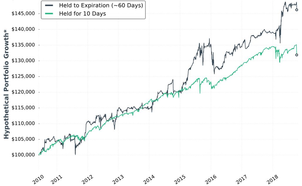
She writes:
> Note: Please ignore the dollar returns in these simulations.
> Pay attention to the general strategy performance. The last
I have wondered about how to interpret these graphs since the second one was presented at the end of Part 7.
> piece we’ll discuss is sizing the positions and we’ll look at
> historical strategy results with various portfolio allocations.
This suggests the graph is done without regard to allocation. With the strategy sized for one contract, I’m guessing the y-axis numbers to be arbitrary yet sufficient to fit the PnL variation. This also means I cannot get meaningful percentages from the graph. As an example, the initial value could be $100,000,000 or $100,000 and still show all relevant information. The percentages would differ 1000-fold, however.
I will now leave you with the following question: as seen above, what unexplained change was made to the graph format that frustrates me most?
Categories: System Development | Comments (0) | Permalink