Debugging the Missing Time Spread Backtrades (Part 3)
Posted by Mark on January 17, 2023 at 06:41 | Last modified: June 27, 2022 19:03I will continue with the debug journey after explaining the complexity of date formats.
As discussed near the end of this post, the date field is in “number of days since Jan 1, 1970.” Although unreadable on its own, I keep this format to check the data file. This can also be subtracted to get difference in days.
While the Python in the link converts these dates to a common format, I have also needed to convert in reverse. I came up with the following for this purpose, which [I think] needs time and datetime modules to work:
int( time.mktime ( datetime.datetime.strptime ( summary_results [ “Trade End” ].iloc [ -4 ], \
“%Y-%m-%d” ) . timetuple ( ) ) / 86400 )
The code takes YYYY-mm-dd as input and outputs days since 1/1/70. I also started to log row numbers in btstats to better identify what rows are matching should I need to refer back to the data file.
I think I am better prepared to approach this debug now that I can convert date forward and backward.
Let’s return to the end of Part 2 where I discovered no apparent problem is being had with the number of matching options.
My next thought was that maybe the particular spread is not being selected from the encoded data. I therefore moved the debug line just below the block where short option variables get assigned:
for i in range ( len ( dte_list ) ):
if dte_list[ i ] >= ( 30 * mte ):
Again, dates_without_enough_matches is empty. So far, things are seeming to work just fine when I know they’re not.
I then added these lines near the top before the conditional block begins to determine control branch:
if current_date != current_date_prev: #debug
print ( f ‘ current_date is { current_date }, common date is { datetime.utcfromtimestamp ( current_date * \
86400 ).strftime( “%Y-%m-%d” ) }, trade status is { trade_status }, and control flag is { control_flag } . ‘ )
current_date_prev = current_date
The idea here is to print out a trace line every time current_date changes (and to update current_date_prev to current_date).
Take a close look at two anomalies that stick out in the following output segment:
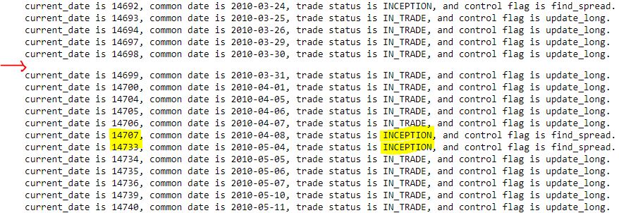
First, I am not sure why I get the occasional blank line as indicated by the red arrow. Current date is always five digits, common date is always the same format, trade_status is at most nine characters, and control_flag is always 11 characters. I get roughly 3500 total trace lines (from 2007 through 2021). In case the trace may occasionally exceed one line in length (thereby showing up as a blank second line), I added ‘123456789’ to the end expecting that I might see many more blanks (or second lines with some of those extra digits). This has no effect; the output looks the same.
While the first anomaly remains unresolved, the second anomaly (yellow) is more relevant. Per this this fourth-to-last paragraph, I am getting some consecutive trace lines printing out with ‘INCEPTION,’ which may indicate missing trade dates. 26 days are skipped from 2010-04-08 to 2010-05-04, though, when I would expect a trace line for each date in the data file.
What is going on here?
Categories: Python | Comments (0) | PermalinkDebugging the Missing Time Spread Backtrades (Part 2)
Posted by Mark on January 12, 2023 at 06:22 | Last modified: June 27, 2022 13:16By way of review, the idea is to log relevant variables in places where spreads could or should be found and aren’t. I left off discussing where in the program I need to insert code to do this.
In case I want to log in the ‘find_spread’ branch, let’s review the sub-branches:
- if int(float(stats[2])) > 200:
I don’t want time spreads with options > 200 DTE. Skipping these rows is expected and no reason to log variables. - elif len(dte_list) == 0 and if int(float(stats[6])) % 25 == 0 and if int(float(stats[6])) > float(stats[3]) and int(float(stats[6])) – float(stats[3]) < 26:
This sub-branch appends data for the option with first matching strike price. It’s always possible that no match will be found in any row for a particular historical date, which to me would suggest an incomplete data file. - elif int(float(stats[2])) == dte_list[0]: continue
This skips rows [on same current_date and] with DTE equal to a previously-matched DTE. Nothing to log here. - elif int(float(stats[1])) == current_date and if int(float(stats[6])) == strike_price:
This sub-branch records DTE for subsequent strike price matches. The different DTE represents a different expiration month. If the previously-matched strike price is not matched here, then it may be evidence of an incomplete data file. - else:
This sub-branch should be executed only after the program has gone through all options on current_date. If no spread has been found, then a skipped trading day will result and len(dte_list) should be < 2. Alternatively, a found spread(s) may not selected in this sub-branch. Either way, logging relevant variables here seems to make good sense.
What are the relevant variables to log?
I increasingly suspect len(dte_list) should be looked at first. On any given day it should be > 2 for at least two matching options (one potential spread). As a first attempt, I will append current_date to a new list dates_without_enough_matches at the top of the ‘find_spread’ ELSE sub-branch for any day that does not meet this criterion.
Surprisingly, the list is empty! This suggests failure to match strike price is not the issue.
Just to be transparent, I am now moving the following line to the end of the ‘find_spread’ ELSE sub-branch:
current_date = int(float(stats[1])) #updating
Since the previous elif executes on the same current_date (and strike price match), by implication this sub-branch takes place on the next day. Updating current_date at the beginning of this sub-branch forced me to use “current_date – 1” in following lines, which may not be accurate in case of weekends, holidays, etc. Updating at the end eliminates this problem. While not part of the current debugging effort, in scrutinizing this part of the program I saw opportunity for improvement.
I will continue next time.
Categories: Python | Comments (0) | PermalinkDebugging the Missing Time Spread Backtrades (Part 1)
Posted by Mark on January 9, 2023 at 06:14 | Last modified: June 24, 2022 11:25Because the current debugging effort is challenging, today I want to put my thoughts to computer screen and push forward to find out why the backtester is missing trades (last discussed here).
Need some juice today? Let’s get in the mood with this (thanks Frida!).
The first thing I should do is run the backtest a couple more times to make sure the values from the table in the previous post are repeatable. I would be more concerned if trades get missed randomly than regularly.
Next, I want to know the values of all relevant variables when trade skipping takes place. I can then trace what I expect should be the logic through the program to see if the results actually match.
Relevant variables can be monitored in one of two ways.
First, I can create a variable containing current_date minus previous trade ending date and raise an exception > 5. This would limit study to one case at a time, which should be sufficient if the cause of missing trades is uniform. Going this route, I need to write the dataframes to .csv and file.close() before raising an exception, which will immediately halt the program. The former will allow me to view the entire dataframe in Excel, which is easier than viewing with Jupyter Notebook. file.close() will avoid the annoying “file in use” warning when I try to open the file after an exception has been raised.
The second way to monitor relevant variables is to let the program run all the way through and collect data on the variables for every trading day without a position. Going this route, I can add code to write to btstats per usual. Skipped days would be evident as consecutive rows labeled ‘INCEPTION.’ I can also scroll down to the particular dates I anticipate this to occur, where I would expect to see mostly zeros with all variables reset.
I’m not sure btstats contains all the relevant variables I want to monitor, which I need to think carefully about to determine. Should this be true, I can always create another dataframe with relevant variables as column names.
The next thing I need to figure out is where in the program I need to call for the relevant variables to be logged. I feel confident to say it should come when control_flag is ‘find_spread.’ That is, after all, when the program is iterating through days without any positions. I also think it makes sense to log relevant variables when spread legs are not encoded.
I will continue next time.
Categories: Python | Comments (0) | PermalinkFinal Word on Formatting Datetime Axes
Posted by Mark on January 6, 2023 at 06:42 | Last modified: June 22, 2022 10:26Today I will pick up plotting datetimes with uniform tick labels.
I’ve learned this is not as difficult as I may* have suspected. The x-coordinates are given in trade_list, which is a list of strings. I need datetimes, which can be created like this:
trade_dates_as_datetime = [datetime.strptime(i, “%Y-%m-%d”) for i in trade_list]
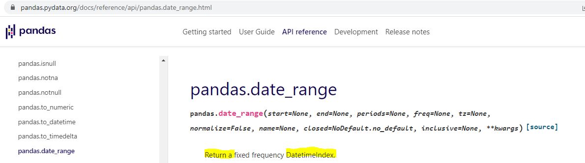
Alternatively, I can ago back to pd.date_range() (introduced here) and include the first/last [string] dates from trade_list:
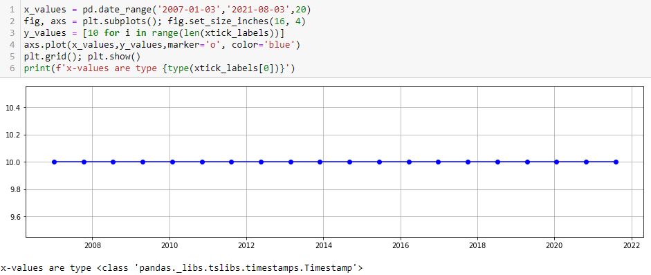
As mentioned in that earlier post, these x-values are type pd.Timestamp, which I believe is a datetime.
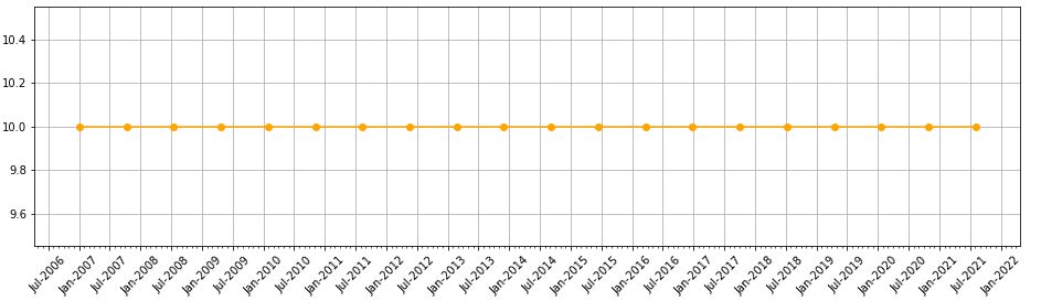
One thing I don’t like is the first major tick printing after the first point. I can remedy with the following:
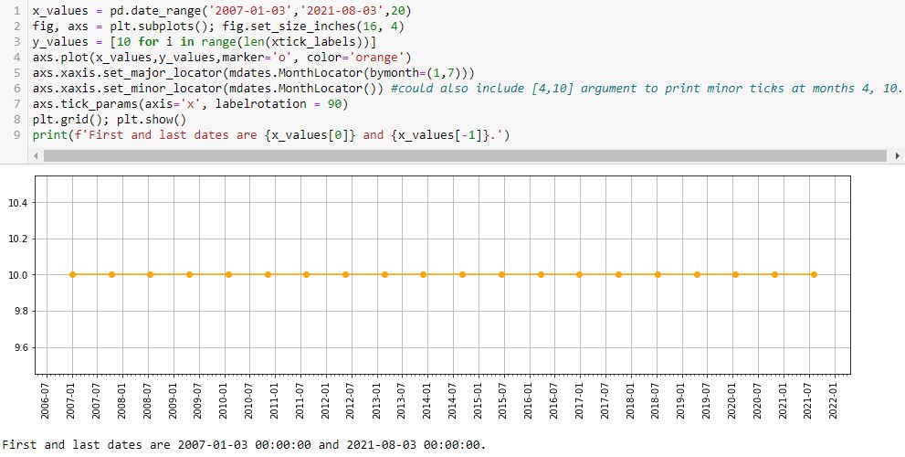
L5 prints major ticks at months 1 and 7. The first (last) major tick is the one preceding (following) the first (last) data point at 2006-07 (2021-08). This is default and leaves ample room to be aesthetically pleasing.
L6 prints minor ticks every month. If so desired, I could specify particular months by including them as a list (e.g. [4,10] would place a minor tick at the other two quarters).
Interestingly, if I put bymonth=(2,6) in L5, then I get something looking like the nasty asymmetry seen in this lower plot:
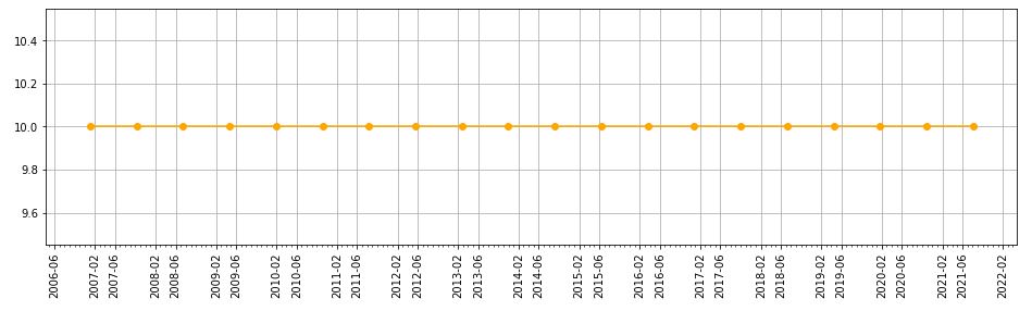
This asymmetry is with major ticks plotted at the same months, though, whereas the earlier one results from major ticks being plotted on the first and 22nd of every month.
With L7 allowing me to adjust rotation, I can now customize about everything I would want on this graph.
Oh—what if I want to put a three-letter month instead of number? I can add this line:
axs.xaxis.set_major_formatter(mdates.DateFormatter(‘%b-%Y’))
Editing rotation to 45 [degrees] produces this:
* — “May” because this has confused and led me in a complete circle to find a complete solution.
Categories: Python | Comments (0) | PermalinkBacktester Development (Part 10)
Posted by Mark on December 30, 2022 at 06:49 | Last modified: June 22, 2022 08:36I stumbled upon a couple further bugs in the second half of this post. Today I want to at least get started on the first one.
All of this started with the graph below and the highlighted point:
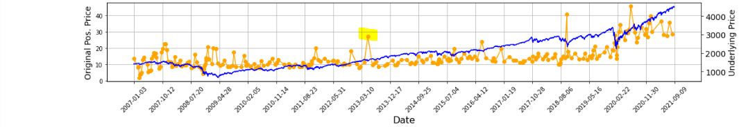
In looking to verify that [locally outlying] trade price, I expected to find early Apr 2013. In fact, the trade in question begins on Jun 21, 2013. Alarmed by the discrepancy, I suspected although the graph appears okay being packed with 255 points (trades), a closer look may reveal the points to be misaligned with dates.
Before going any further, I really should have checked to see if this is true (it is). Let’s do that right now:
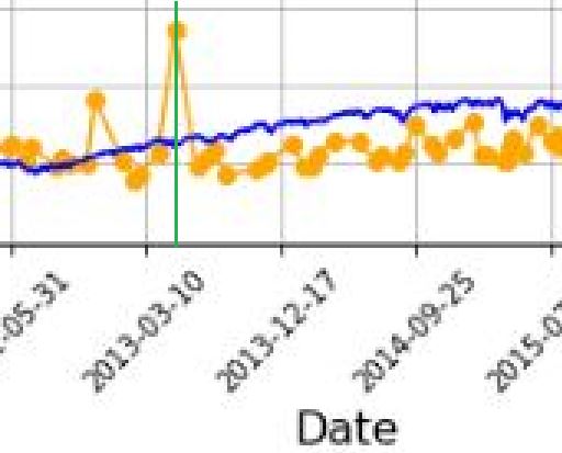
I added a green, vertical line with MS Paint and calculated the distance between the green line and the previous vertical grid line (3-10-2013) as a fraction of the distance from the previous and following (12-17-2013) vertical grid lines. The fraction is 0.208, which places the date at May 5, 2013. The point is off by 47 days. That may not be much for a graph that spans over 14 years, but I thought computers didn’t make mistakes?!
It then occurred to me that while successfully getting the x-axis tick labels horizontally spaced, the points on the graph are also uniform even though the intervals between dates are not.
Once again, before going any farther I should have checked to see if this is true. Look closer at the second graph. Does the horizontal spacing look even to you? To me it doesn’t, but how can I verify?
I could do something like this:
P_price_orig_zeroes = [ 0 for i in P_price_orig_all ]
axs[1] . plot ( trade_list, P_price_orig_zeroes, marker=’o’, color=’g’ )
This creates a shadow line to the orange with equal x-values but all y-values set to zero:
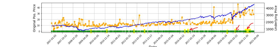
Along the green line at the bottom, I have highlighted in yellow (punctuated by a few red arrows in case the highlighting is unclear) where the points are farther apart and the green line exposed.
As it turns out, the points do not align with dates but the horizontal spacing is not uniform, either. I now suspect the latter is due to the second bug I mentioned in the link from the first paragraph.
With regard to a possible cause for the irregular spacing, the code uses ax.set_xticks(). This is similar to plt.xticks() for which I included some documentation here. Looking closely at the former:
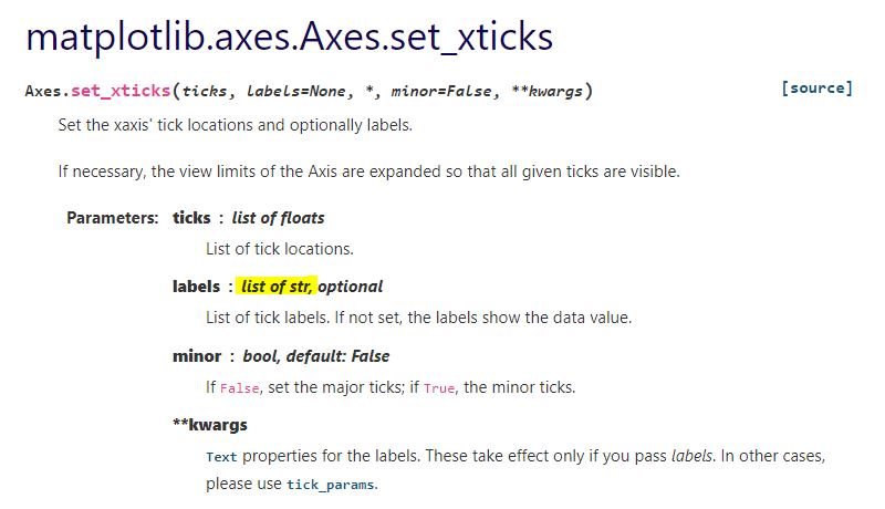
This establishes a list of strings as tick labels. Failure of the points to correctly align with label values (dates) makes sense for arbitrary strings as opposed to meaningful datetime objects. For correct alignment, maybe I can’t use ax.set_xticks() at all.
I want to correctly plot datetimes, but I want uniform tick labels rather than labels only where x-coordinates exist to match.
How can I make that happen?
Categories: Python | Comments (0) | PermalinkTime Spread Backtesting (Part 2)
Posted by Mark on December 27, 2022 at 06:25 | Last modified: June 23, 2022 14:26Last time, I began easing into time spread backtesting with my Python automated backtester by discussing trade verification. Before getting into that, I need to flush out a couple bugs in the program.
Because sudden equity jumps in the first graph may be seen as other anomalous prints on the other three graphs, I will begin with the three outlier position prices seen on the second graph. The first appears to be ~$30 around the beginning of Apr 2013. As an original price, this should be visible in the summary file:
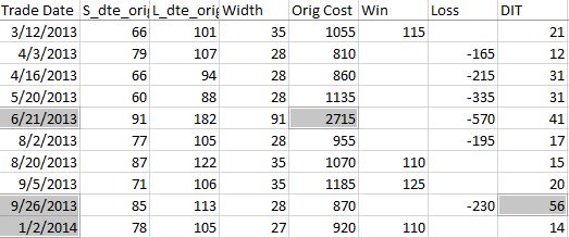
Although the trade in question is obviously from 6/21/13 ($27.15 * 100/contract = $2,715 original cost), it plots closer to the beginning of Apr 2013. I think the problem is everything I did here with regard to “plots the evenly-spaced date labels at evenly spaced locations on the x-axis.” Unfortunately, the trades are not evenly-spaced. Although I want the tick marks to be evenly spaced in time and distance across the graph, I want the x-values of the points to correctly match the x-axis.
This will need fixing.
Another problem regards the final trade of 2013 beginning Sep 26 and lasting 56 days. Rounding off, the next trade should begin around Nov 26 (two months later). Surprisingly, the next trade does not begin until Jan 2, 2014. What happened?
I am tempted to think any open trade at the end of a year gets erroneously junked in favor of a new trade beginning first trading day of the following year due to an iteration technicality.
However, the anomaly does not seem to reduce to anything that consistent. It does not repeat for 2014 (trade ends Dec 19 with next trading starting Dec 31). It is not applicable for 2015 (Dec 22 trade correctly carries over to Jan 7, 2016) or beyond. Going backward from 2013, the anomaly does present in 2012 and in 2010.
To pin this down more accurately, I replaced the Trade Date column in summary_file with Trade Start and Trade End columns. In Excel, I then subtracted the previous Trade End from Trade Start and sorted this Date Diff column from highest to lowest. Because I was missing the previous trade ending date, I inserted that as a new column making sure to Paste Special by values to prevent sorting triggering a recalculation:
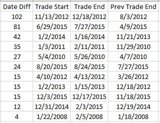
Date differences of four or less are within normal limits. One would be a new trade starting on a weekday after the previous trade ended yesterday. Two could be a weekday market holiday such as Independence Day coming in between. Three would be a new trade starting on a Monday after the previous trade ended on Friday. Four would be a trade ending on a Thursday or Friday with new trade starting the following Monday or Tuesday due to a Friday or Monday market holiday.
I could even stretch to explain a five in case the market were closed for an extended period. For example, due to Hurricane Sandy the markets were closed Monday, Oct 29, and Tuesday, Oct 30, 2012.
As shown above, the list skips from four straight to 12. This defies any explanation. If the data files are clean, then I expect entries and exits on back-to-back trading days every single time.
There’s something going on…
Categories: Backtesting, Python | Comments (0) | PermalinkTime Spread Backtesting (Part 1)
Posted by Mark on December 22, 2022 at 06:39 | Last modified: June 13, 2022 14:30Bumps and bruises are still to come along the road ahead, but Version 14d of my backtester is at least somewhat functional. I am now ready to start presenting and interpreting results.
Let’s start with something very basic. In rough terms, SPX_ROD1 time spread strategy is as follows:
- If flat, then open one contract with short leg 2-3 months to expiration and long leg 4-5 weeks farther out in time.
- Exit trade if ROI% > +10% profit target or ROI% < -20% max loss.
Here are the results:
- 257 trades
- 196 winners (~76%)
- Average profit $221
- Average loss $383
- Profit factor of 1.86
In case this seems like a legit backtest, be aware of some things that are missing:
- Trade verification
- Exploration of time stops
- Exploration of alternative exit levels
- Max excursion analysis
- Drawdown analysis
- Position sizing
- Transaction fees
Looking at a summary line in isolation hides a lot of critical information. Things like cost, DIT, width, closing PnL—pretty much anything, really—should be evaluated in relation to surrounding trades to reveal potential errors. I may have coded incorrectly, or I may have a corrupt data file. I have not done my due diligence if I can’t verify by looking through a trade one day at a time to check for reasonable consistency. This isn’t to say I need to look through every trade in every backtest every time, but I should at least do some periodic spot checking.
I already have some means to do this spot-check verification. I have two output files with summary and intratrade statistics as well as four graphs [shown below in two separate screenshots] that I spent a lot of time debugging (e.g. this mini-series):
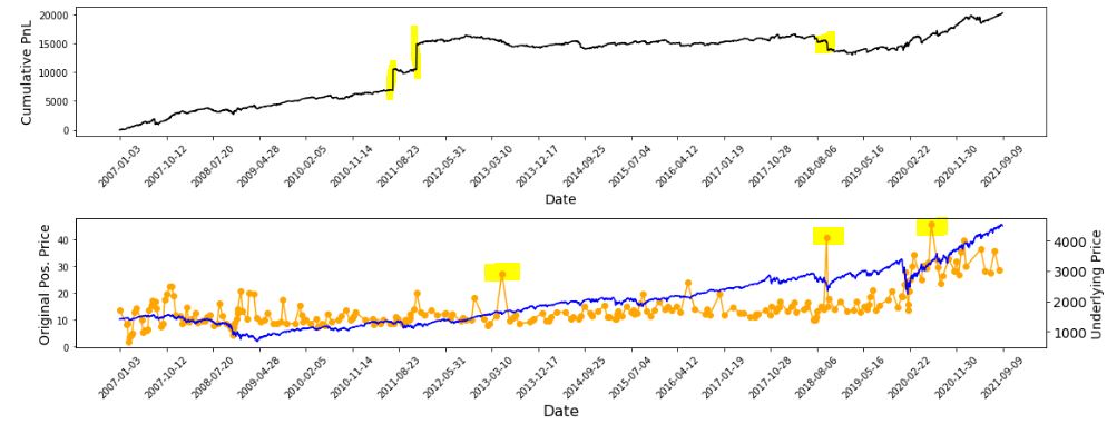
The first graph is an equity curve. Any sudden jumps are things that I want to inspect. I have highlighted three. I remember summer 2011 as a volatile market. I’m not sure about mid-2018. I will take a closer look at the trade log.
The second graph shows trade prices in orange. Any significant spikes are worthy of investigation to make sure nothing more than isolated volatility is responsible for the short-term outlier. I have highlighted three spikes on the graph.
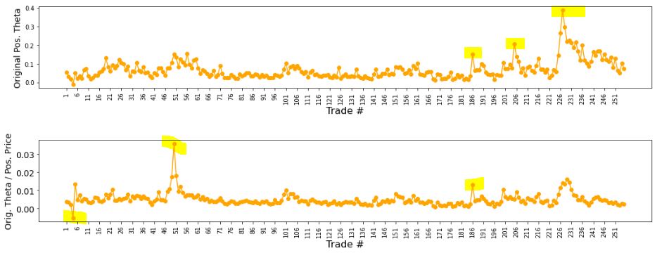
The third graph shows position theta at trade inception. I have highlighted three spikes worthy of a closer look.
The final graph normalizes initial position theta by trade cost. I have highlighted three spikes that are worthy of investigation. The first of these is clearly below zero, which suggests either theta or cost starts out negative. I can hardly imagine either one of those given accurate data so I definitely want to analyze that.
I will continue next time.
Categories: Backtesting, Python | Comments (0) | PermalinkBacktester Development (Part 9)
Posted by Mark on December 19, 2022 at 06:29 | Last modified: June 22, 2022 08:37Today I want to finish updating what I have for backtester logic beginning with other considerations regarding maximum excursion (ME; see end of Part 8).
I’m not convinced that I need to report ME in btstats. As the statistic itself refers to an intratrade value, I can only think of two reasons to include it in the intraday report: to see how it changes over the course of the trade, which doesn’t matter to me, or to see exactly when it occurs, which I know anyway because I store that number separately ( _dte). All the context I probably need is in summary_results where I will also see initial DTE and DIT.
Besides, comparing ME across trades is easy in summary_results but much more difficult in btstats. In the former, each row corresponds to one trade and looking at ME across trades is as simple as scanning from row to row. In the latter, multiple rows correspond to each trade and I would need to do a lot of scrolling and looking up ‘WINNER’ or ‘LOSER’ in trade_status.
Removing ME from btstats will simplify an if-elif-else to if-else since ‘WINNER’ and ‘LOSER’ are otherwise handled the same.
And if trade_status is ‘WINNER’ or ‘LOSER,’ then before continuing data file iteration the program proceeds to:
- Assign ‘INCEPTION’ to trade_status
- Assign ‘find_spread’ to control_flag
- Reset all variables (fifth-to-last paragraph of Part 7 aside)
- Assign True to wait_until_next_day
I added a profit factor calculation to summary_results by:
- Appending two more rows (dictionaries) for mean and count of wins and losses by doing
summary_results = summary_results.append ( { } ) [not just summary_results.append()] - Calculating PF_calc by using .iloc[ ] to look up particular values
- Appending a row at the bottom to display PF_calc
Finally, I once again had to debug the graphing portion having to do with the x-axis tick labels that I discussed here, here, here, and here. I end up resolving this with three lines:
L1: xtick_labels = pd.date_range (btstats [‘Date’] . iloc[0], btstats [‘Date’] . iloc[-1] , 20 )
This creates a list of 20 evenly-spaced trading dates including the first and last.
L2: xtick_labels_converted = xtick_labels . strftime ( ‘%Y-%m-%d’ )
This is needed to avoid ConversionError [“Failed to convert value(s) to axis units”] from L3.
L3: axs[0] . set_xticks (list (np . linspace (1, len (btstats . index), num = \
len (xtick_labels_converted) ) ), xtick_labels_converted, rotation = 45)
This plots the evenly-spaced date labels at evenly spaced locations on the x-axis.
Technically speaking—and these are the details on which I get hung up and confused as a beginner—pd.date_range() in L1 returns a Datetimeindex. How do we know that and what does it mean?
I can do an internet search for pd.date_range:
I can do an internet search for datetime index:
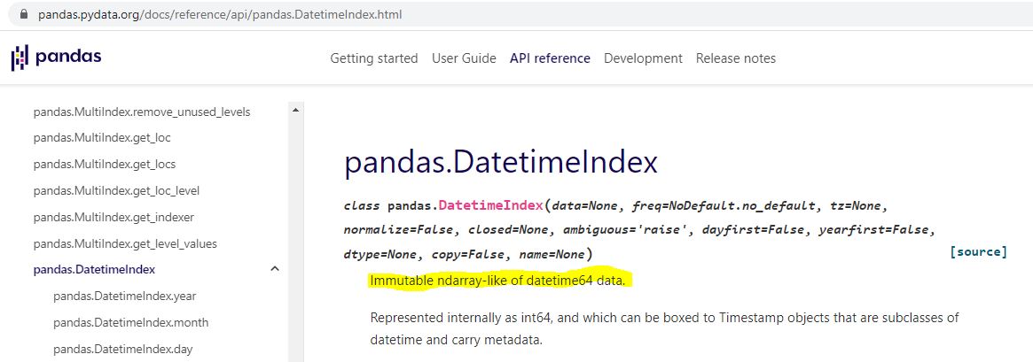
Is “ndarray-like” bad English? An internet search turns up a page that explains this, too.
Ndarray can also be better understood by an internet search:

I don’t know much about arrays yet, but I do know they are a different data type from what [an internet search has informed me that] ax.set_xticks() is expecting:
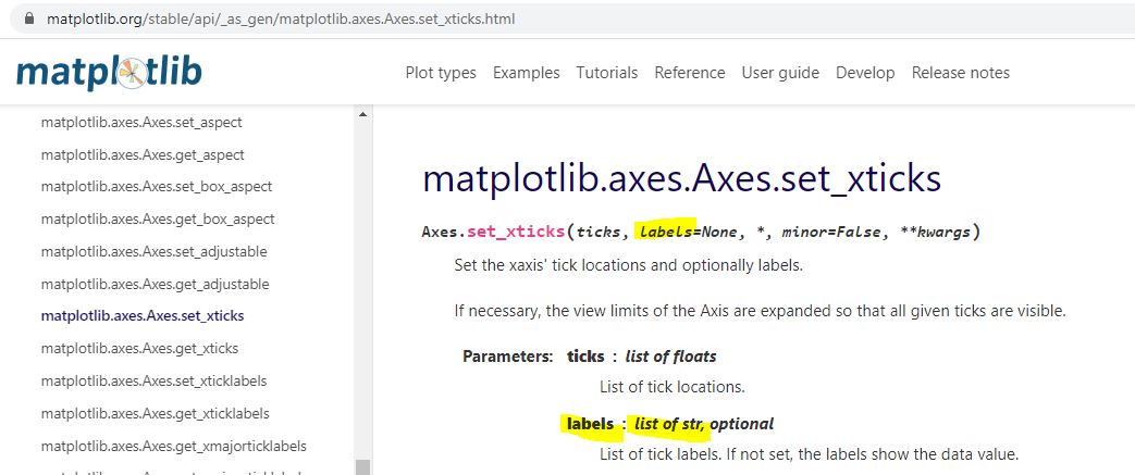
Type str[ing] rather than [type] array or Index is expected. The Datetimeindex has large integers that nobody would want to see as tick labels anyway. L2 converts those to strings with a familiar character format (YYYY-MM-DD).
That pretty much covers the updated logic for this version of the backtester.
Categories: Python | Comments (0) | PermalinkBacktester Development (Part 8)
Posted by Mark on December 13, 2022 at 07:02 | Last modified: June 22, 2022 08:37Today I will continue (see end of Part 7) with backtester logic for maximum excursion (ME).
I will begin talking about the output files. Two dataframes are created with pd.DataFrame(): btstats for intratrade monitoring and summary_results for end-of-trade reporting. These are ultimately converted to .csv files with pd.to_csv().
Rows are added sequentially to the dataframes upon completion. For btstats, add_btstats is created where each list element corresponds to a dataframe column. Minimal calculation in this list statement (e.g. L_iv_orig x 100) could have been done with variable assignment if I renamed the variables to reflect it. Index of the last record is then used to add list to the bottom:
> btstats.loc [ len ( btstats . index ) ] = add_btstats
In contrast to adding rows as lists, I build summary_results by adding rows as one dictionary per trade:
> summary_results = summary_results . append ( { ‘Trade Num’ : len (trade_list) }, ignore_index = True)
This is a long line with a key-value pair for every column (only one of which is shown here). The final argument is needed when appending a dictionary to avoid a TypeError.
Pandas documentation says DataFrame.append() has been deprecated in favor of .concat(). I do not get any such warning. A closer look suggests the deprecation pertains to adding one dataframe to another. I am adding a dictionary.
Now that I have described the structures in which ME will be reported, let’s talk about ME itself. By definition, MFE (favorable) is the farthest a trade goes in my favor before ending up a loser and MAE (adverse) is the farthest a trade goes against me before ending up a winner. Strictly speaking, a losing (winning) trade has no MAE (MFE).
However, a useful application might involve running trades from start to finish without profit targets or max losses to record largest intratrade loss and gain. Plotting the two against each other can then give an idea whether a particular stop level might lock in more winners to the exclusion of losers or avoid locking in more losers to the exclusion of winners. All this is contingent on knowing whether intratrade gain or loss comes first. I have the _dte variables to tell me that.
To allow for such application, I define MFE (MAE) to be maximum intratrade gain (loss) without regard to trade outcome. My tweak is to recognize MFE (MAE) for winning (losing) trades as the previous day’s MFE (MAE) before stop level is hit.
Needing to differentially apply current or previous ME when stop levels are checked after ME is updated makes the program logic more complicated. For trade_status ‘IN_TRADE,’ I report MAE and MFE. For ‘WINNER’ (‘LOSER’), I report MAE and MFE_prev (MAE_prev and MFE). All this leaves me with three different add_btstats lines that need to be properly fit into an if-elif-else block. The same goes for summary_results.
I will continue next time.
Categories: Python | Comments (0) | PermalinkBacktester Development (Part 7)
Posted by Mark on December 5, 2022 at 07:16 | Last modified: June 22, 2022 08:37Today I will finish discussing the ‘find_spread’ control branch before moving on to ‘update_long.’
A few final steps are taken after the spread is identified:
- All variables are assigned from lists.
- First row of btstats (intratrade_results) is added.
- trade_status is changed to IN_TRADE.
- Control flag gets assigned ‘update_long.’
- Several variables and lists are reset. This includes converted_date.
- Break out of the for loop.
The last step is critical. I initially included a continue statement, which repeats the loop and selects the longest-dated option under 200 DTE every time: definitely not what I want.
I’m somewhat confused in determining where the program goes next, but I think it must be back to the top of the data file iteration loop. The for loop, of which this is a part, concludes the ELSE of the ‘find_spread’ control branch. Unlike the previous version, at this point the program is already looking at the next date so nothing needs to be done with wait_until_next_day.
The ‘update_long’ branch is brief. If strike price and long expiration date match, then variables for the long option are updated along with underlying price. If strike price and expiration date do not match, then continue to the next line of the data file.
I am sloppy with what variables to reset at the end of ‘find_spread.’ Some variables not reset are used in ‘update_long.’ What matters most is that every variable to be subsequently passed to btstats gets assigned a new value as part of the update branches. I’ve discussed possibly using functions to initialize and reset variables. Much of the resetting (and initializing) is unnecessary as long as I assign everything at the proper points. I try and reset where I can since I don’t trust myself with this, but I could shorten the program simply by being more careful.
The ELSE, which executes when control_flag is ‘update_short,’ begins with a check to make sure current_date still matches historical date. False would indicate the spread failed to be updated: a fatal flaw.
Next and similar to above, if strike price and short expiration date match, then variables for the short option and the spread are updated. No need to change underlying price as date has not changed.
I then include logic for max adverse/favorable excursion. I need variables for MFE, MAE, MFE_dte, and MAE_dte. I also need to store the previous values because I never want the max excursion to be equal to closing PnL.* If ROI_current < MAE (or > MFE), then the MAE (MFE) values get assigned to a _prev variable set and ROI_current gets assigned to MAE (MFE).
I will continue next time.
*—Alternatively, I could have used and maintained lists with two elements
each rather than duplicating the variable set with a _prev suffix.