2021 Performance Review (Part 2)
Posted by Mark on March 29, 2022 at 06:47 | Last modified: February 8, 2022 11:23Last time, I began to lay the groundwork for a long-term performance review. Today I will continue the discussion.
My hopes for doing this in Python resulted in the project dragging on for a couple extra weeks until I finally decided to stick with my original Excel spreadsheet, which had data from 2001 – 2016. The first thing for me to do was to complete this through 2021. The first few months of the spreadsheet looks like this:
![]()
Eventually, I started adding the last Friday dates for the beginning and end of the monthly periods to make lookup quicker.
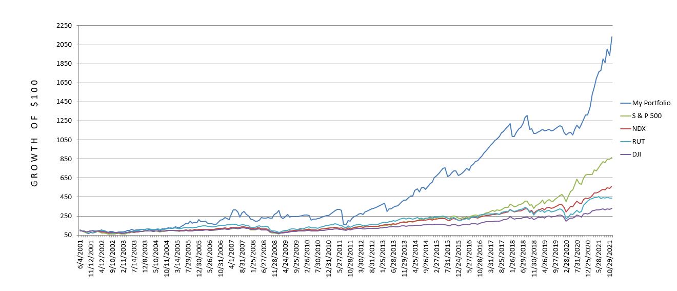
After entering the monthly performance of my portfolio through 2021, I calculated monthly performance for SPX, RUT, NDX, and DJI. As the spot indices do not include dividends, I fetched historical dividend yield data from http://www.multpl.com/s-p-500-dividend-yield/table for SPX and https://www.macrotrends.net for the other three. On the latter website, IWM and QQQ yields are provided quarterly and DIA yields monthly. For each data series, I took the highest value for all four quarters (or 12 months) and used that as the dividend yield for the entire year.
As a result of this conservative manipulation, the benchmark return is slightly enhanced and my comparative trading performance will be weaker. I prefer to err on the side of conservativism (see sixth paragraph here and last full paragraph here) just in case I’m ever caught wearing the rose-colored glasses without my notice (e.g. sixth paragraph here).
I also seize the opportunity for conservatism in my handling of missing QQQ yield data. No data are available prior to 2006. I therefore plugged in the highest quarterly yield recorded from 2006-2021 for 2001-2005. The gist of all this is to weaken my results when reasonable to do so. If I still come out shining bright then it may be a significant finding. I feel the same way about backtesting performance: bias against backtesting results in every way possible such that if the results still pass muster, I may indeed be looking at a viable trading candidate.
I have discussed critical analysis many times (e.g. third-to-last paragraph here). To believe something is worthwhile in this industry, performance results should be impressive beyond a reasonable doubt. Make sure to include the headwinds because you can be sure Mr. Market won’t forget them (see fifth-to-last paragraph here) at the hard right edge of the chart.
Here’s a first look at the performance comparison:
I will continue next time.
Categories: Accountability | Comments (0) | Permalink2021 Performance Review (Part 1)
Posted by Mark on March 24, 2022 at 06:59 | Last modified: February 7, 2022 10:20Today I begin a mini-series to update my trading performance through 2021.
I haven’t done a performance update in a while, but I should do this every year. My first such review began with this post. Four years later I did this one. Later that year I also did this post with some nice graphs and data. The following year I did this one. Finally, I did this one to finish up a draft I had begun months earlier. This post includes some performance notes.
2021 was my best trading year ever. One could say I was lucky. Then again, as traders we are always lucky whenever a different market environment would have resulted in a much worse outcome. This is especially the case when the superior performance is realized in the face of an improbable (subjectively defined) market environment.
I tend to be reluctant to take credit for things I do not control. I do not control the market, but I am the one doing the trading and for that I deserve credit. Certainly if my account tanks, I will always get the blame by my own worst critic (for starters).
Some of this is about humility, which is a topic I have written about or alluded to in the last paragraph here, this post, this mini-series, this mini-series, this post, and this mini-series where I gave a very honest and open evaluation of myself.
Aside from reviewing my 2021 trading performance, in what follows I will go back to 2001 and recalculate the numbers relative to different indices factoring in dividend yield and tax differential for active trading. I incur a 60/40 blended tax rate compared to the benchmarks, which for purposes here will be considered LTCG. I don’t have a CIPM®, but I think any accurate performance comparison should address this point.*
Because my original plan was to crunch numbers in Python, this has become more of an ordeal than anticipated. My spreadsheet breaks down monthly periods by the last Friday of each month being the starting point for one period and the ending point for another. Not every Friday is a trading day (holidays), though, which means I sometimes use Thursday values. I’m fine giving a Friday date even when there is no trading on that day because it’s still a true statement. In some extreme cases, we may have had no trading on a Thursday and a Friday. Programming all this can get rather involved.
I will continue next time.
* — If you start reading performance reports, I think you will come to the realization that most do not.
Time Spread Backtesting Concepts (Part 3)
Posted by Mark on March 21, 2022 at 07:21 | Last modified: January 11, 2022 13:55Today I conclude this brief mini-series detailing background concepts about time spreads.
Theta is one parameter I found insidious in manual backtesting. 2020-2021 time spreads generally have a lot of “jump.” They seem to hit profit targets quickly and sometimes completely out of the blue (e.g. with PnL small or negative just a day or two beforehand). 2017 time spreads, in contrast, move very slowly. Weeks go by without any significant profit and loss is more common. Perhaps because I monitored the TD ratio per guidelines shown here, I did not think to track theta itself.
2017 volatility is extremely low and I eventually realized that position theta is extremely low with these guidelines, too. Over a given period, the market can be expected to move within a probability cone. When theta is much lower, profit will not accumulate to offset this movement. Without normalizing theta by adjusting spread width, these guidelines really describe entirely different strategies for 2017 and 2020/2021. As shown in the table here, width will affect MR, which can then be normalized as discussed in that final paragraph.
Eventually, I would like to do a study with no profit targets or stop-losses. Track MFE with DTE, MAE with DTE, and then visualize to check for optimal values. This should be done in walk-forward fashion to avoid generalized curve-fitting. Maybe every month I visualize a chart of MAE/MFE over the previous six months to see what values are optimal based on recent history. These values may or may not be stable going forward.
To get started, something simpler like backtesting with a straight 10% profit target and -20% max loss could be done. I should then try to generate a variety of combinations to verify the strategy as profitable in all cases. Other pairs could be 10%/-10%, 15%/-20%, 20%/-20%, 20%/-15%, etc. Of course, the higher the number the longer the trades. For this reason, some measure of PnL%/day also makes sense…
…and by now I have lost the “simpler” part. Keeping complexity out is certainly one of the larger challenges here.
Rewind: start with +10%/-20%. I can then compare strike selection from -5% to ATM to +5% by increments of 1%, 2%, or 2.5% to assess directional bias. Transaction fees should be included, and avoiding less-liquid strikes is a possibility.
As one last piece of theoretical complexity, I suspect an X% change in horizontal skew has less effect on PnL as DTE decreases. Lower DTE means less extrinsic value remains in the short option to be affected by IV change in the first place. Tracking horizontal skew % may therefore be misleading unless done with regard to DTE.
Categories: Option Trading | Comments (0) | PermalinkTime Spread Backtesting Concepts (Part 2)
Posted by Mark on March 18, 2022 at 06:45 | Last modified: January 10, 2022 14:23Today I want to continue with background on time spreads before moving forward with Python backtesting.
How horizontal skew reacts to different types of market rallies and/or selloffs is hard to predict. In selloffs when fear spikes, traders tend to buy near-term options pressuring term structure toward backwardation (increasing horizontal skew). In theory, increased IV is good for vega-positive time spreads. If horizontal skew becomes more positive, then although the long leg increases in value (good) due to IV, short-leg value may increase more (bad). The overall effect on PnL depends on how decreased spread value from higher skew compares with increased spread value from higher long option prices.
You can imagine other permutations for cases where horizontal skew is initially positive or negative, becomes more positive or negative based on different magnitudes of rally/selloff, etc. I am interested to see if any significant association exists between [changes in] horizontal skew and profitability.
I am also interested to see if any significant association exists between IV and profitability. Conventional wisdom says vega-positive time spreads should be purchased when IV is low. Could horizontal skew have a significant interaction here?
Margin requirement (MR) varies from one time spread to another and I have had difficulty putting my finger on this. MR is proportional to IV. MR should be inversely proportional to DTE since all else being equal, time spread price increases over time and maximum potential risk is the cost. Width (days between expirations) is directly proportional to MR because for the same short option, long options farther out in time are more expensive. Horizontal skew should also be inversely proportional to MR because the higher skew means a more-expensive near-term option and lower overall cost.
To simplify things a bit:
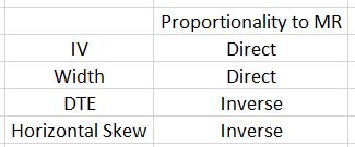
Perhaps Python can aid with some analysis here.
With MR so variable, some consideration must be given to position sizing. One possibility is a fixed position size backtest where each trade is done with number of contracts (rounded down) equal to position size ($) / MR. Alternatively, a fixed percentage of the total account could be allocated. This would allow for compounding. Drawdowns across the equity curve could then be compared as percentages off the highwater mark to normalize for temporal sequence. This seems logical at first glance.
I will continue next time.
Categories: Option Trading | Comments (0) | PermalinkTime Spread Backtesting Concepts (Part 1)
Posted by Mark on March 15, 2022 at 07:00 | Last modified: January 7, 2022 15:44I previously introduced my recent manual backtesting of time spreads that I hope to automate going forward in Python. Let’s back up a bit and discuss some general concepts pertaining to time spreads themselves.
A time spread is composed of a short option in one expiration and a long option at the same strike price in a more distant expiration. I proclaim the primary profit mechanism is differential time decay with short option decaying faster than the long.
Time spreads have delta risk, vega risk, and term-structure risk.
Delta risk refers to the positional tendency to maximize profit over time as the underlying market trades toward the strike price. The [roughly] triangular risk graph illustrates this. At expiration, profit is greatest at the strike price. Above and below, expiration profit wanes until it becomes zero or negative with the market trading sufficiently far beyond the strike.
For a directional time spread placed with current market significantly above or below the strike price, delta risk refers to loss accumulation as the underlying moves farther from the strike or as the underlying remains sufficiently far from the strike as short-option expiration approaches.
Time spreads placed ATM are sometimes referred to as nondirectional. The position can [eventually] profit regardless of whether the underlying moves up or down as long as it remains within a limited range. The ATM time spread still has delta risk because enough market movement away from the strike price either today or by expiration will drive PnL negative.
Vega risk—tendency of a position to lose money due to IV change—exists because the long option, which is farther from expiration, has more extrinsic value than the short. Time spreads are therefore vega positive: as IV increases, the long leg will increase more in value than the short leg will decrease. As IV decreases, the time spread loses value and the expiration curve, which always indicates PnL at short-option expiration, moves down. This is true assuming all else remains the same.
Term structure—the difference in IV between expiration months—often does not remain the same.
Term-structure risk for time spreads refers to an increase in horizontal skew. Horizontal skew is short-option IV minus long-option IV. Horizontal skew is generally negative, which makes positive horizontal skew advantageous for entry.* Should skew revert lower, the short option can lose more extrinsic value than the long, which biases the spread toward profitability. Once a time spread has already been opened, however, increased horizontal skew biases the spread toward loss because short-option extrinsic value increases more than long.
I will continue next time.
*—Always question why horizontal skew is positive as part of your trade assessment.
Practice Trades Cal 1.13
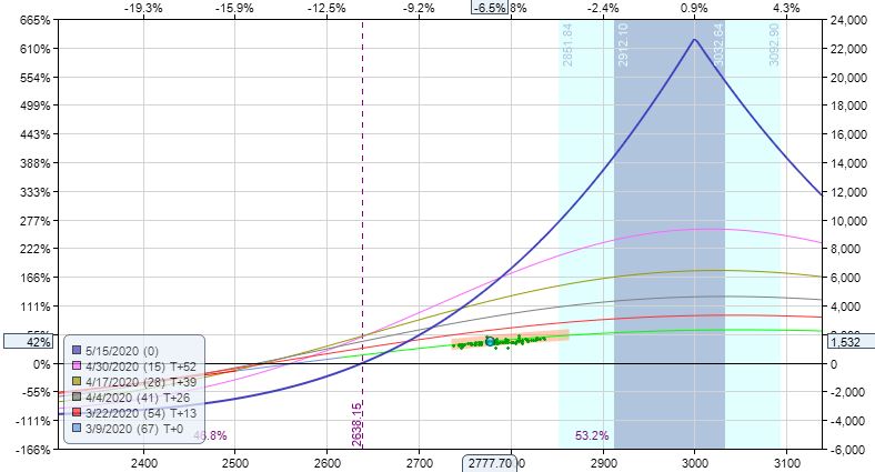
Posted by Mark on March 10, 2022 at 06:21 | Last modified: December 24, 2021 12:28Cal 1.13 (guidelines here) begins 2/18/20 (87 DTE) with SPX 3370 and trade -$168 (-2.6%). TD = 1, MR $6,498 (two contracts), IV 11.9%, horizontal skew -0.85%, NPD 6.8, and NPV 231.
What jumps out at you when looking at the initial risk graph?
This is the second Cal example where the same strike is unavailable in the back month (see Cal 1.4 here). Placing the long leg lower gives the trade a bullish bias, which is something discussed in the fifth paragraph here.
Notice that a bullish bias is achieved whether I diagonalize the long leg (lower) or whether I raise the calendar strike. The former preserves profit potential at current underlying price at the cost of raising MR. Each has pros and cons.
As mentioned in the third paragraph here, I may want to come up with some alternative downside management since TD = 1 at inception unless I plan to let it go to ML.
On 84 DTE, trade -4.4% with market down 0.85 SD in three days.
Exit 81 DTE for loss of $1,478 (-22.8%). This is the 4.33 SD down day, which comes without warning. Over 6 days, SPX down 2.73 SD with IV up 83%. Horizontal skew has increased slightly to -0.62%. TD = 0 (rounded).
Unlike Cal 1.2, SOH to see how the market “shakes out” would be a terrible decision here:
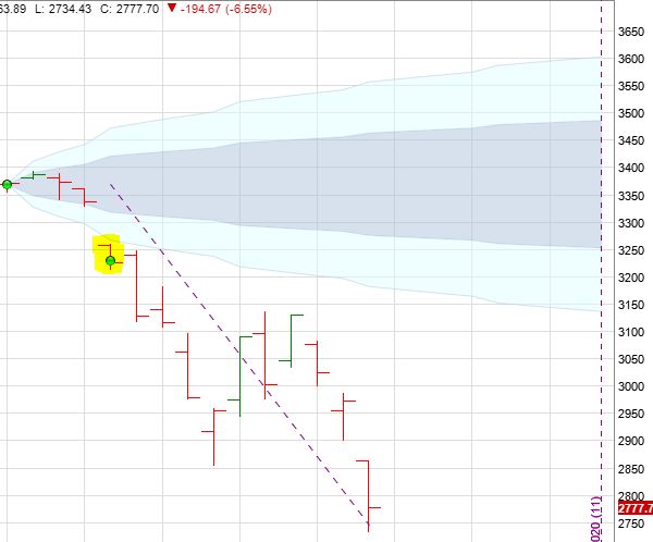
Highlighted is my first opportunity to exit at max loss (with market far outside profit tent and TD 0 unlike third paragraph here where Cal 1.12 is still well-positioned with TD strong). I have to take the loss immediately: no reason not to.
HEED WARNING DISCRETIONARY TRADERS!
I think one of the biggest risks of discretionary trading is the tendency to see something that seems to work while conveniently forgetting other instances where it does not. You may be confident in something that, on the whole, adds no benefit (or worse). A large-sample-sized systematic backtest to assess strategy guidelines can prevent this from happening.
Categories: Option Trading | Comments (0) | PermalinkTime Spread Backtesting in Python (Part 1)
Posted by Mark on March 7, 2022 at 06:35 | Last modified: January 7, 2022 11:33Recently, I did a blog mini-series manually backtesting the COVID-19 crash with time spreads. I left off suggesting backtesting of a slightly rather than extremely bullish time spread as more representative of the long-term market.
One benefit to manual backtesting is a closer look at the day-by-day PnL of each and every trade. Seeing this is a closer approximation to live trading than only seeing the trade result.
Ultimately though, Python is where I want to be for automation, for efficiency, and for all of my backtesting needs. Manual backtesting takes much longer. It also requires me to go back and do many other calculations whenever I want a slightly different look at the data, whenever I want to calculate additional trade statistics, etc.
For me as a beginner, Python has a big temporal cost. That won’t change unless I work consistently to improve my skills.
I want to try and organize my thoughts about this backtesting and maybe come up with a flow chart before I actually try writing any code. I’ve been advised this can help prevent me from getting stranded in the weeds spending lots of time ironing out bugs that aren’t all that important.
This might be a decent time to start transitioning to Python since I’ve been backtesting in ONE and have a fresh sense of what the process entails.
Part of the process I won’t have with Python includes risk-graph management, which is prominently displayed in ONE. Without programming Black-Scholes (way too difficult for my current proficiency), I won’t have any ability to model the trade in Python. I therefore won’t see a profit tent, day steps, or PnL breakevens. I can’t reject the possibility this affects my [manually backtested] Practice Trades, but no risk graph information is called by trade guidelines so hopefully this isn’t an issue.
The .csv data file includes greeks, which will allow for some common techniques of trade management.
To start, I need to think about what I want the program to output and what it will take as input. Here is a snippet of the option data file that gets purchased as .csv archives:
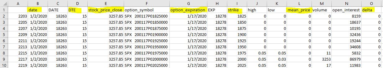
The actual data file has more columns. For time spreads, I will need all greeks but gamma along with IV.
The spreadsheet column headers I have been using in recent manual backtesting provide a starting point for the kind of data I’m looking to collect. Reading down:
Trade #
ONE Trade #
DTE
SPX
MR
Theta
TD
IV
NPD
NPV
MDD %
DTE
Max MR
# Adj
Exit DTE
ROI
SD Chg
IV Chg
DIT
Horiz Skew %
TD
Comments
I will continue next time.
Practice Trades Cal 1.12 (Part 2)
Posted by Mark on March 4, 2022 at 07:12 | Last modified: December 24, 2021 12:34I left off questioning whether I should exit Cal 1.12 at max loss despite being well-positioned inside the profit tent.
From a systematic, programming standpoint, I don’t see how to do breakeven (BE) estimation with time spreads without Black-Scholes and/or volatility skew modeling. This precludes implementation of a Python backtester.
From an “art of trading” standpoint, my gut says “no way no how” do I take max loss when I am well inside the profit tent (strongly supportive of a high TD) like this.* To convince me otherwise, I will be on the lookout for cases where I remain in such trades only to meet a horrific demise.
Exit two trading days later at 73 DTE for profit of $552 (15.3%). SPX is up 0.13 SD to 3011 with IV up 5.9% over the 5 days, TD = 96, and horizontal skew remaining at +1.8%.
Part of me wonders if it might require extraordinary discipline to exit still being positioned near the center with TD so high.
If I stayed in, then when would I look to exit?
Moving ahead to 11 DTE:
I am now approaching the downside BE. While still 140 points away, I am certainly getting to the “slim pickins'” portion of the graph compared to what lies to the right. TD is 10 at this point and trade is +42.5%, which would be an absurd amount to lose should the market continue lower.
This would be a decent time to exit. I may not be able to code this discretionary interpretation, but said “art of trading” still seems alluring as a viable tool.
Finally, I’m a bit curious about the margin requirement (MR). I mentioned in this third paragraph that high IV may cause time spreads to be expensive. Such is not the case with Cal 1.12. I will grant that Cal 1.12 IV (~35%) is nowhere near that seen in Cal 1.3, but it still seems relatively high whereas MR seems relatively low. With starting DTE, horizontal skew, and [average] IV [proprietarily calculated over the whole option matrix in ONE] all potential contributing factors, how can this be explained?
I will pick up here next time.
* — This is 31.3% of the way between BEs.
Practice Trades Cal 1.12 (Part 1)
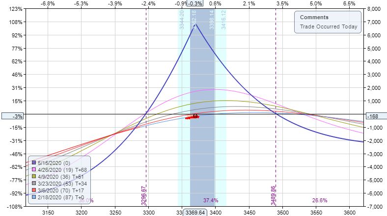
Posted by Mark on March 1, 2022 at 07:06 | Last modified: December 24, 2021 12:34Cal 1.12 (guidelines here) begins 2/27/20 (78 DTE) with SPX 2995 and trade -$168 (-4.3%). MR is $3,608 (two contracts), TD 53, IV 35.2%, horizontal skew +1.8%, NPD 0.8, and NPV 224.
“Conventional wisdom” (see second paragraph) would probably suggest skipping this day for entry given a crazy market down 3.1 SD! I can imagine a volatile, whipsaw market causing hefty slippage, but looked at another way if I place a limit order and just wait, then I can imagine having a good chance to be filled precisely because of the market’s wild movement.
The positive horizontal skew provides me with a little extra bonus compensation for the risk taken in a volatile market.
How much compensation, you ask?
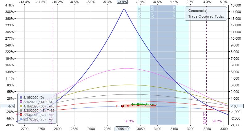
I admittedly zoomed in to make this look super large. However, what is no joke is 460 points between expiration breakevens (BE)—a full 15% of the underlying’s current price. If volatility tanks then the graph will move down and BEs will narrow, but as the positive skew reverts, T+0 will rise. Lots of moving parts here.
Surprisingly [to me], the official max loss (-$728, -20.2%) is hit the very next day with market down 1.1 SD:
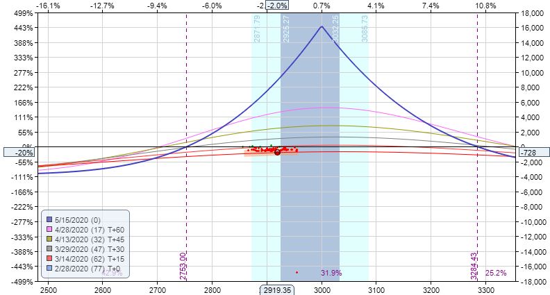
Should I exit this trade?
The market is down 59 points, but I still have 166 points to downside BE. Distance between expiration BEs has increased to 530 points with IV now at 45.4%. Horizontal skew has increased and I still expect a reversion to negative horizontal skew to follow (recall last paragraph here). TD 25 also suggests solid potential for profit potential going forward.
I will continue next time.
Categories: Option Trading | Comments (0) | Permalink