Trading System #1–SPY VIX (Part 5)
Posted by Mark on October 16, 2012 at 06:40 | Last modified: October 5, 2012 07:07The subjective function is now in hand: RAR/MDD. I will now recreate the results presented in http://www.optionfanatic.com/2012/10/02/trading-system-1-spy-vix-part-3-2 and redo the consequent analysis.
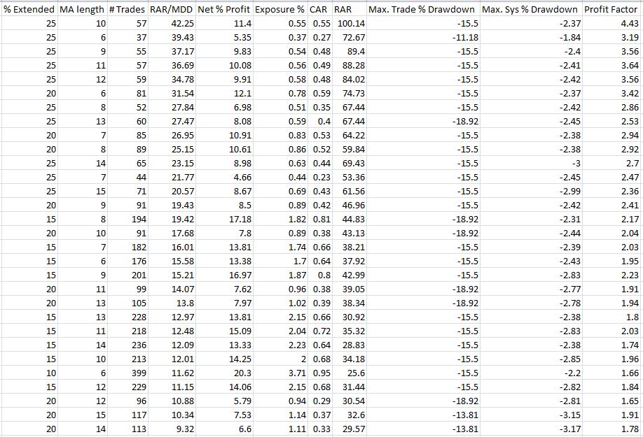
Here are the results for the top 30 parameter combinations as sorted by RAR/MDD:
My first observation is that a cluster of 25% extended systems sit right at the top. Indeed, running a linear regression analysis on all 50 systems shows that % extended and RAR/MDD are correlated with an R-squared value of 0.77 (R-squared > 0.80 is typically considered “strongly correlated”).
This makes logical sense as a mean-reversion trading system. Mean-reversion systems are based on the idea that the farther the rubber band gets stretched, the more likely it is to snap back [to the mean]. The more extended VIX gets above or below the VIX moving average, the more likely SPX is to move higher or lower, respectively. This was also seen [less clearly] in the graph of Net Profit % (http://www.optionfanatic.com/2012/10/03/trading-system-1-spy-vix-part-4/).
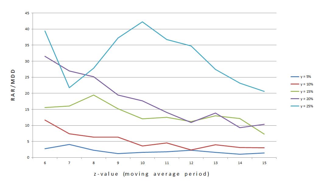
If I break down systems by z-value (moving average period), then the results look like this:
Keeping in mind that I want to see plateau regions rather than spike regions, the bottom curve (y = 5%) looks best. The statistics do not bear this out, however:
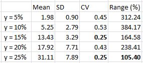
Table 2
Mean = average RAR/MDD
SD = Standard Deviation
CV = Coefficient of Variance (SD / mean)
The lower the SD, the flatter the curve. Even more important is to interpret SD as a percentage of the mean since the means vary over 15-fold. By that metric, y = 25% is the most consistent.
Indeed, y = 25% has a greater RAR/MDD over the entire range of z values. Even the lowest RAR/MDD for y = 25% (at z = 7) is greater than the highest RAR/MDD for y = 15% (at z = 8). Given these observations, y = 25% seems to be the best choice.
I will continue this analysis in the next post.
Categories: Backtesting | Comments (0) | PermalinkMotion to Dismiss System Development?
Posted by Mark on October 15, 2012 at 06:07 | Last modified: October 4, 2012 06:38I now have the subjective function from http://www.optionfanatic.com/2012/10/12/the-subjective-function-part-6/. Before I move on and apply this to the SPY VIX trading system, I want to briefly discuss one other point that threatens to derail system development.
In my last post (see above), I mentioned the following with regard to high-profit, infrequently-trading (i.e. “surgical”) systems:
> Ideally, I would like to take advantage of the time one such system is not in the market
> by trading with another surgical system that is in the market. I am therefore in the
> market more frequently with systems that deliver concentrated profits.
When trading with surgical systems, the only way to achieve a reasonable percent return on the entire portfolio in a risk-controlled manner is to combine them.
Statistically speaking, this is the employment of non-correlated systems (i.e. low R-squared values). With two non-correlated systems, one system may be making money while the other is flat (i.e. out of the market) or one system may be losing money while the other is making a bit more. The catch is that R-squared is calculated based on historical data. During explosive market conditions, one system may make money when the other system suddenly loses much more. Even worse, both systems may become correlated and lose money together.
While these are threatening possibilities, without more details I can’t say it’s reason to dismiss system development altogether. You could look at a long historical backtesting period to determine how often these conditions occur. When they occur may be generalizable to a particular type of market condition. You could explore the possibility of including a failsafe filter–for example, suspending trade of a mean-reverting system in case of powerful breakout or breakdown. Whether the markets traded by these systems are the same or different could also affect the severity of this threat.
I will continue analysis of the SPY VIX trading system in my next post.
Categories: System Development | Comments (0) | PermalinkThe Subjective Function (Part 6)
Posted by Mark on October 12, 2012 at 04:51 | Last modified: October 1, 2012 06:31I unmasked the systems in yesterday’s post (http://www.optionfanatic.com/2012/10/11/the-subjective-function-part-5). Prior to that I made all my observations about the graphs shown in http://www.optionfanatic.com/2012/10/09/the-subjective-function-part-3. Once and for all, the time has arrived to select the subjective function.
On one hand, I like a system that trades more and presents more opportunity for profit. This sort of system has a profit factor (PF) just over 1.00 and grinds out a small profit in each of many trades. This would be insert #3.
On the other hand, I prefer systems that are surgical in their efficacy. These generate infrequent trades and have larger PFs (e.g. over 1.50 or 2.00). Ideally, I would like to take advantage of the time one such system is not in the market by trading with another surgical system that is in the market. I am therefore in the market more frequently with multiple systems that each deliver concentrated profits. I prefer this model.
The risk of using surgical systems to make the equivalent dollar profit as a frequent trading system is that larger position sizing must be employed. Although the likelihood is that these trades will end up profitable, in case the next trade results in MDD the larger position size could result in catastrophic loss.
I want a subjective function that takes into account both profit and DD. A system may have had minimal DDs in backtesting but as one author on system development described, your worst DD is always ahead of you. If the subjective function does not factor in DD then I fear the Risk of Ruin.
Therefore, I will choose RAR/MDD (insert #1) as the subjective function. By using RAR instead of compound annualized return, I also like the fact that the more a system is out of the market, the more it is rewarded.
Categories: System Development | Comments (1) | PermalinkThe Subjective Function (Part 5)
Posted by Mark on October 11, 2012 at 09:05 | Last modified: January 18, 2013 07:59Yesterday in http://www.optionfanatic.com/2012/10/10/the-subjective-function-part-4, I began the analysis of graphs posted in http://www.optionfanatic.com/2012/10/09/the-subjective-function-part-3 to determine the subjective function. Today I will make my remaining observations.
Equity curve #3 posts the greatest profit of all three curves. This profit of 20.3% is roughly 283% greater than equity curve #2 and about 78% greater than equity curve #3. This relates to my previous observation of also being in drawdown (DD) more than the other two. If curve #3 is in DD more than the others but is drawing down from a much greater net profit then I may still be happier with this system than with the others.
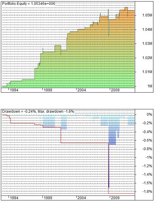
With regard to maximum DD (MDD), insert #2 has the edge. MDD here is -1.8%, which is 25% less than insert #1 (-2.4%) and 18% less than insert #3 (-2.2%). Lower DD means less risk. I could increase position size a bit to make for comparable MDDs and a larger profit for insert #2. While this suggests I could increase position size slightly, though, it certainly would not make up the 283% greater profit equity curve #3 has over #2.
Do not forget that in order to secure the 283% profit, insert #3 has over 10 times as many trades as insert #2 and is therefore in the market over 10 times longer. Theoretically, this is greater risk that could turn sour on us in the future even though it did not significantly do so in 19.5+ years of backtesting.
Time to unmask the systems:
–Insert #1 (y = 25, z = 10) generated the highest profit factor of all 50 systems.
–Insert #1 generated the highest risk adjusted return (RAR).
–Insert #1 generated the highest RAR:MDD ratio.
–Insert #2 (y = 25, z = 6) is the system that generated the lowest MDD.
–Insert #3 (y = 10, z = 6) is the system that generated the highest net profit.
So which is better?
Categories: System Development | Comments (1) | PermalinkThe Subjective Function (Part 4)
Posted by Mark on October 10, 2012 at 07:31 | Last modified: October 1, 2012 06:03I’m in the process of trying to determine the subjective function, as defined in http://www.optionfanatic.com/2012/10/05/the-subjective-function-part-1. In http://www.optionfanatic.com/2012/10/09/the-subjective-function-part-3, I showed three inserts to help us in this determination. I will analyze those today.
Let me start by emphasizing the need to study relative differences in net profit, drawdown, and other details between the three inserts. If I focus on absolutes then I will be disappointed. The one and only goal of this study is to determine which I prefer most.
In looking at the equity curves, my first observation is that they are all upward sloping to the right. I should hope so. Each insert corresponds to the system that performed best on a different metric. Whichever curve I like the best corresponds to the metric I will use to evaluate systems. This will be the subjective function. Since each of these systems is the best in some respect, I am glad to see they are all profitable.
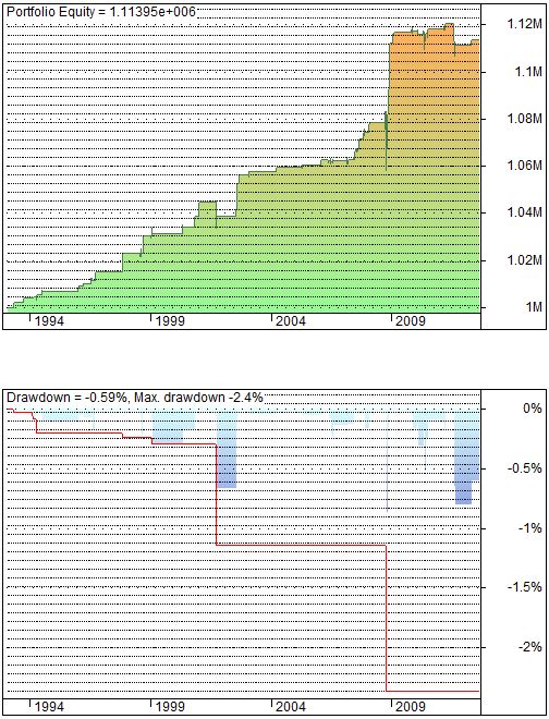
Equity curves #1 and #2 have many discernible plateau (horizontal) regions as opposed to #3, which seems to have more incremental changes. This corresponds to the total number of trades. Inserts #1, #2, and #3 have 57, 37, and 399 total trades, respectively. On this metric alone, I prefer a system that trades more because that means more opportunity for profit.
Drawdown curves #1 and #2 have a much smaller blue area than #3. This means #3 spends more time in drawdown and less time at new equity highs. I really like new equity highs because they make me feel like a successful trader. The broad market does not make all-time highs very often.
Equity curve #1 is lower now than it was around the beginning of 2009. This seems like a negative. However, each of these systems goes into drawdown periodically and curve #1 did hit a new high roughly 1+ centimeters ago (on my screen), which is only a couple fractions of a centimeter more than the other two. Curve #1 just happens to be in greater drawdown (-0.59%) than the other two but by no means it this drawdown remarkable. This observation may be disregarded.
I will continue this analysis in my next post.
Categories: System Development | Comments (2) | PermalinkThe Subjective Function (Part 3)
Posted by Mark on October 9, 2012 at 05:37 | Last modified: September 28, 2012 07:30I keep coming up with quirky analogies for different aspects of the system development process. In http://www.optionfanatic.com/2012/09/19/trading-system-1-initial-assessment-part-1/ on 9/19/12, I talked about a Motion to Dismiss. On 10/8/12 (http://www.optionfanatic.com/2012/10/08/the-subjective-function-part-2), I talked about visiting the eye doctor. As promised, today I will present some graphs for study to help determine the subjective function.
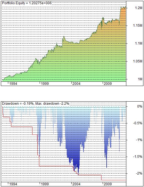
The following inserts show two graphs each. On the top is the equity curve itself: a plot of account value over time beginning with $1M and traded with a $100K position size. On the bottom is the drawdown (DD) curve. DD is zero whenever the account is at a new high. The red line on this graph tracks the max DD ever seen over the whole time period. You will see the red line dip to levels not seen in the blue graph but that is only because the DD was too short to be seen in the blue graph. If you were able to zoom in and magnify then you would see the blue graph dip to those levels.
As you look the following three inserts, imagine that you are studying the performance of your investment account over time. Which would you feel best about? Note details such as relative net profit (final value is shown in the upper left of the top curves), relative severity of drawdowns (current drawdown at the right edge of the bottom curves is shown in the upper left of the bottom curves), relative time between new equity highs, number of horizontal periods (indicating no current trade), etc.
Now without further ado, let me present…
Insert #1:
Insert #2:
Insert #3:
I will analyze these graphs based on my preferences in the next post.
Categories: System Development | Comments (1) | PermalinkThe Subjective Function (Part 2)
Posted by Mark on October 5, 2012 at 17:25 | Last modified: October 4, 2012 06:35My last post (http://www.optionfanatic.com/2012/10/05/the-subjective-function-part-1) defined the subjective function. Today I want to present another perspective on the subjective function by explaining what I previously missed.
The gist of my previous posts is that all traders are looking for the same general thing. “Consistent profitability over time” is a phrase I have written many times over. Yes, Trader A may be looking for the supercharged exponential returns that carry the risk of heavy drawdowns while Trader B is more conservative and will sacrifice returns to minimize drawdown. Aren’t they both basically looking for consistent profitability over time, though?
No.
I now see that Trader A and Trader B are looking for decisively different things. My “consistent profitability over time” is what Trader B seeks. Trader A, however, is in effect buying a lottery ticket and hoping for the big payout. If financially savvy then Trader A is playing this with a limited percentage of the total portfolio so as not to go completely bankrupt. Trader B might be all-in with proper asset allocation.
My previous lack of understanding might reflect an inadequacy of language itself. I suspect we just don’t have enough terms to reflect the variety of individual preference for investment returns. Compound annual growth rate (CAGR), drawdown (DD), and flat times translate directly to features seen on equity curves but others do not (e.g. profit factor, Sharpe and Sortino ratios). Equity curves reflecting the same CAGR or DD can look wildly dissimilar, however. The pictures tell more than words can describe.
Moving beyond language in this manner is what Dr. Bandy recommends in Quantitative Trading Systems (2007) to determine the subjective function. After running the trading system optimization, scroll through the different equity curves to find the ones you like best. Note which metrics score highest on your favorite equity curves and voila! You have the subjective function. This is not unlike a visit to the eye doctor where you endure an exhausive series of “which lens is better: one or two? 1 or 2? 2, or 1? 2, 1?”
In fact, let’s do that: a visit to the optometrist’s office, and more, when we return.
Categories: System Development | Comments (1) | PermalinkThe Subjective Function (Part 1)
Posted by Mark on October 4, 2012 at 19:03 | Last modified: October 4, 2012 06:34I’ve mentioned multiple times that in trading system development we’re looking for consistent profitability over time. To do this, identification of the “subjective function” is a prerequisite.
Much of the direction to my current work is owed to Dr. Howard Bandy. You can read about him here: http://www.linkedin.com/pub/howard-bandy/b/b44/270 . In his book Quantitative Trading Systems (2007), Bandy defines the “objective function” as:
> A single-valued measurement of the fitness of a trading system. Optimization
> techniques are guided by maximizing the value of the objective function.
He also writes:
> Only you can decide which trading systems are good and which are not.
> Selection of the objective function is a management decision and must
> be made prior to extensive model development. The objective function
> itself is not a candidate for optimization.
What does this mean?
System trading is the epitome of Yin and Yang! Beginning on 5/7/12 (http://www.optionfanatic.com/2012/05/07/strategies-vs-systems-part-i/), I wrote a number of blog posts discussing discretionary vs. systematic trading. The upshot was that discretionary trading is subjective and systematic trading is objective. This may be true but at the heart of a somewhat objective system development process is the very personal selection of Bandy’s objective function. For this reason, I have chosen to call it the subjective function.
All this subjective function talk may seem highly theoretical but it really boils down to something quite simple. On 10/4/12 (http://www.optionfanatic.com/2012/10/04/trading-system-1-spy-vix-part-4/), study the y-axis to see my subjective function: net profit (%). I proceeded to discuss the best combination of parameters by performance on that measure.
The only problem is that I failed to go through the process of determining my subjective function before implementing it.
Stay tuned for further discussion and a possible detour in upcoming posts.
Categories: System Development | Comments (3) | PermalinkTrading System #1–SPY VIX (Part 4)
Posted by Mark on October 3, 2012 at 23:03 | Last modified: October 4, 2012 06:32Today I will begin to analyze results of the SPY VIX trading system optimization study. Please refer to Tables 2A and 2B from http://www.optionfanatic.com/2012/10/02/trading-system-1-spy-vix-part-3-2 for the backtest results.
My first observation is that each of the 50 parameter combinations leads to a profitable system! Net profit % ranges from 4.66% to 20.30%. Remember that the issue we’re ultimately trying to address is how probable it is that the system we are backtesting will generate profit going forward. All parameter combinations backtesting profitably makes me more confident that the chosen system will be profitable in live trading than if all parameter combinations did not backtest profitably.
While this conclusion may seem obvious, it does head off the tendency to infer more from the observation than is actually presented. Beginning (and seasoned!) traders are all-too-often eager to enter the market with any half-decent excuse for a [potentially] winning system, open their bags, and let the money fall in. This is the allure/mirage of Wall Street (otherwise known in human nature terms as “greed”). The harsh reality is quite to the contrary. It takes great effort to develop profitable systems and we have just begun. Perhaps “all backtested systems profitable” is one of our checkpoints but our checklist better be much longer if we are to have a realistic chance of being good and not lucky (or worse).
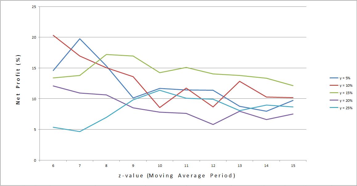
Following the course of evolutionary operation, I now want to analyze returns of each y-value individually:
What line(s) has large plateau regions rather than spike regions? The red line seems to dive early (e.g. from z = 6-10) and then flatten out. The blue line goes up and then way down before flattening. The green line seems relatively flat. The light blue line rises early on and then retraces half that rise. The purple line falls gradually but seems pretty flat from z = 9-15.
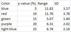
This eyeball method is consistent with a cursory statistical analysis:
Green and purple lines vary the least (flatness).
The one problem I have with this method is the percentage nature of the dependent variable. That is, falling from 20(%) to 15(%) or 10(%) to 5(%) are both a range of 5% but the former is a 25% difference whereas the latter is a 50% difference.
That criticism aside, based on these data I would choose y = 15% and z = 10 (near the middle of plateau regions).
I will continue this analysis in future posts.
Categories: Backtesting | Comments (1) | PermalinkTrading System #1–SPY VIX (Part 3)
Posted by Mark on October 2, 2012 at 08:01 | Last modified: September 21, 2012 09:21In http://www.optionfanatic.com/2012/10/01/trading-system-1-spy-vix-part-2/ (10/1/12), I continued the discussion of evolutionary operation by reviewing optimization. Today I will begin the optimization process for the trading system.
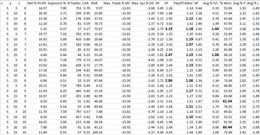
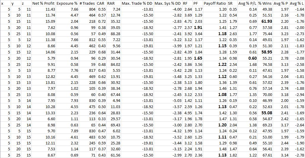
For the initial backtest, I am going to leave x fixed at 5 days and, as mentioned in the last blog post, vary y from 5-25 in increments of five [e.g. 5 (percent), 10, 15, 20, or 25] along with z from 6-15 in increments of one. Other backtesting assumptions were discussed in “Trading System #1–Backtesting Assumptions” from 9/14/12. The only change here is that I will take long and short SPY trades when VIX is “overbought” and “oversold,” respectively.
Table 2A
Table 2B
I abbreviated headings to make the Table font larger:
CAR = Compound Annualized Return (%)
RAR = Risk Adjusted Return (%) = CAR / Exposure %
Max. Trade % DD = Largest intratrade drawdown (%) (denominator is position size)
Max. Sys % DD = Largest portfolio drawdown (%) (denominator is current account value)
RF = Recovery Factor = Net profit / Max. System DD (higher is better)
PF = Profit Factor
Payoff Ratio = Average win / Average loss (second term of PF calculation)
SR = Sharpe Ratio
Avg % P / L = Average % gain or loss per trade
Avg % P = Average % profit on winning trades
Avg % L = Average % loss on losing trades
Several trends are evident from studying these results. The numbers in bold and larger font are unexpected values with regard to these trends. Feel free to take some time to peruse the Tables.
In my next post, I will begin the data dissection.
Categories: Backtesting | Comments (2) | Permalink
