Trading System #1–SPY VIX (Part 1)
Posted by Mark on September 28, 2012 at 05:31 | Last modified: October 1, 2012 05:35With the “motion to dismiss” now denied, the next step is to lay the groundwork for developing this strategy into a trading system.
As a review, the trading strategy is based on two claims. First, five days after the CBOE Volatility Index (VIX) closes 5% or more below its 10-day simple moving average (SMA), the S&P 500 index (SPX) has lost money on average. Second, when the VIX closes 5% or more above its 10-SMA, SPX has outperformed the average week better than 2-1 over the next five trading days.
The current system in development offers three variables to be backtested: x-bar stop y% extended from its z-SMA. In this case, we have used x=5 (five-day trades), y=5, and z=10 (VIX closing 5% above/below its 10-SMA). What we want to see in backtesting is solid results with these values. We also want to see solid results when we slightly change these values, though.
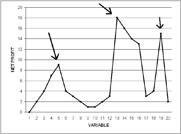
The process of “evolutionary operation” looks to keep one variable constant while changing another to see its effect on system performance. Graphically speaking, we want to plot some measure of performance (e.g. net profit) vs. the one variable being changed:
This does not have the appearance of a robust system because slight changes in the variable drastically affect net profit. Whether a moving average is four periods vs. five or 14 periods vs. 15 should not matter. If one value appears magically improved in the midst of mediocre results then those backtested profits are likely a matter of luck rather than the system taking advantage of consistent opportunity (and subsequent future profits).
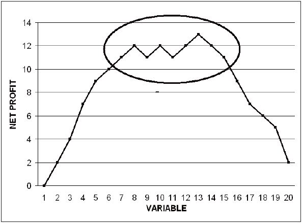
This is what we hope to see. All values from 6-15 produced solid profit for this trading system. Rather than the spikes in the previous graph we see a plateau region in this one. This should be a necessary (but not sufficient) condition for a system we might trade in the future with real capital.
These graphs were adapted from Tomasini and Jaekle (2009).
In my next post I will continue this discussion in terms of optimization.
Categories: System Development | Comments (2) | Permalink
Trading System #1–Initial Assessment (Part 6)
Posted by Mark on September 27, 2012 at 06:38 | Last modified: September 21, 2012 06:55In my post http://www.optionfanatic.com/2012/09/25/trading-system-1-initial-assessment-part-5/ (9/25/12), I finished up my analysis of the overbought VIX trading strategy. Today I want to study the claim of avoiding SPY when VIX is oversold, which I described in http://www.optionfanatic.com/2012/09/13/trading-system-1-introduction/ (9/13/12).
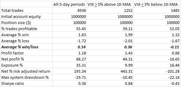
Do 5-day long trades in SPY actually lose money if placed when VIX is over 5% or more below its 10-SMA (“oversold”)? I have included these results in the third column in order to compare with all 5-day SPY trades and 5-day SPY trades only when VIX is “overbought”:
Indeed, the oversold VIX strategy loses money. Average % win is much smaller (1.32%) and the lower % trades profitable (52.05%) contributes to a negative profit factor and negative Sharpe ratio.
Now having substantiated both of the initial claims, I feel more confident about putting forth time and effort to try and develop a trading system. I will continue with these steps in my next post.
Categories: Backtesting | Comments (0) | PermalinkTrading System #1–Initial Assessment (Part 5)
Posted by Mark on September 25, 2012 at 07:09 | Last modified: September 21, 2012 06:54We have been studying the difference between 5-day long trades in SPY with daily entry vs. with entry only when VIX closes at least 5% above its 10-SMA (“overbought”). Going back to Table 1 from my post http://www.optionfanatic.com/2012/09/19/trading-system-1-initial-assessment-part-1/ (9/19/12), today we will discuss the remaining results.
The overbought VIX strategy gets a slight edge with regard to % profitable: 59.11% to 55.45%. In a broad sense, systems are usually trend-following or mean-reverting (i.e. sell when the market is strong and buy when the market is weak). Trend-following systems typically have a lower % of profitable trades whereas mean-reverting systems have a higher % of profitable trades. Trend-following systems typically have a much better average % win (for winning trades) to average % loss (for losing trades) ratio, however. This is the tradeoff. Recall that % profitable trades and average gain/loss are the two components of profit factor (PF) calculation.
The final statistic is the one I highlighted with bold: average % win/loss. In looking at Table 1, this statistic seemed to be the coup de grace for the “overbought” VIX strategy. With both strategies having similar winning percentages, the “overbought” VIX strategy dominated with a 0.36% vs. 0.14% average % win/loss. This difference is also reflected in the PF although the difference is not as clear (1.43/1.18 << 2). The difference is reflected in the SR but as previously discussed SR is shroud in more complexity and controversy as a meaningful number. One needs to have studied many systems before developing an intuitive understanding of how SR differences may reflect system performance.
In my post http://www.optionfanatic.com/2012/09/13/trading-system-1-introduction/ (9/13/12), I mentioned the internet claim that “when VIX closes 5% or more above its 10-SMA, SPX has outperformed the average week better than 2-1 over the next five trading days.” Based especially on this average % win/loss statistic, I consider that claim to be verified.
This now leaves us to determine SPX (SPY) performance when VIX is “oversold.” I will address this in the next post.
Categories: Backtesting | Comments (2) | PermalinkTrading System #1–Initial Assessment (Part 4)
Posted by Mark on September 24, 2012 at 06:20 | Last modified: September 19, 2012 06:12Today I will continue to compare the SPY daily long strategy with vs. without an overbought VIX filter by discussing Sharpe Ratio (SR).
The Sharpe Ratio (SR) is one of the most commonly referenced measures of risk/return. It is calculated as the difference between the average return and the risk-free rate divided by the standard deviation of all returns.
The numerator of the SR describes “excess return.” The better the average return of the system the greater this number will be. The sign of SR will be determined by the numerator and any potentially profitable system must have a positive SR.
The denominator rewards systems that have higher consistency of returns. Typically when a system performs well, positive returns are consistent (e.g. closing at set profit targets). When the market goes awry for a system, feel lucky if you get taken out at your stop-loss point. In many cases with violent market moves, a gap may jump far beyond a stop-loss point before the trade closes. For this reason, more poorly performing systems have a larger variability of returns and therefore larger denominator.
A primer on how to calculate SR with Microsoft Excel is seen here: http://investexcel.net/214/calculating-the-sharpe-ratio-with-excel/ .
The SR has been highly criticized in financial circles and should therefore be taken with a grain of salt. For one thing, rewarding consistency of returns (e.g. 2% per month rather than 12% one month and 0% the other 11 months) means short option premium strategies often get high SRs. Short option strategies have catastrophic risk, however, that many other trading strategies do not (think Long Term Capital Management in 1998). What is also debatable is that the SR penalizes variability of returns whether that variability is profit or loss. A strategy that returned 2% in 11 months and 12% in one month would reflect similarly in the denominator as one that returned 2% in 11 months and -8% in one month.
In the current study, buying SPY when VIX is “overbought” results in a much better SR of 0.84 vs. 0.36. As is often the case with other system statistics, SR is often negatively correlated with exposure. This means in order to get the desired net profit out of your portfolio, a single highly profitable system won’t be enough. The goal should be to find multiple systems with large PFs or large SRs to work together.
Categories: Backtesting | Comments (0) | PermalinkTrading System #1–Initial Assessment (Part 3)
Posted by Mark on September 21, 2012 at 05:54 | Last modified: September 21, 2012 06:51In my last post http://www.optionfanatic.com/2012/09/20/trading-system-1-initial-assessment-part-2/ (9/20/12), I focused on the concept of drawdown (DD) in the current backtest. Today I want to analyze Profit Factor (PF).
In my opinion, PF may be the most critical system statistic to study. PF is defined as:
# winning trades average gain
————————- x ———————-
# losing trades average loss
Stated differently, PF is how many dollars are gained per dollar lost.
A profitable system will have a PF > 1. If PF < 1 then the system loses money. An outstanding system prospect will have a PF > 2.
PF should be studied in conjunction with exposure. In many instances, PF and exposure are inversely proportional. A system may have an outstanding PF but trade only once per month. That will likely not give you sufficient profit to trade unless you trade the system really large. This would be too risky with regard to the possibility of Ruin.
Table 1 (http://www.optionfanatic.com/2012/09/19/trading-system-1-initial-assessment-part-1/) shows that the average 5-day SPY trade generated a PF of 1.18 vs. 1.43 for all 5-day SPY trades commencing on a VIX close at least 5% above its 10-SMA. This suggests the latter is a more profitable system, but as discussed in my last blog post, exposure is smaller. As I also discussed, max DD is smaller, which may enable us to trade larger. Column 3 shows the larger position size also generates the higher PF along with a higher net profit %.
I hope you are gaining an appreciation for the complexity of system development. Many statistics must be analyzed together and in reference to each other. Even when that is done, different conclusions can be made depending on what is most important to the individual trader.
Categories: Backtesting | Comments (0) | PermalinkTrading System #1–Initial Assessment (Part 2)
Posted by Mark on September 20, 2012 at 05:55 | Last modified: September 21, 2012 06:48In http://www.optionfanatic.com/2012/09/19/trading-system-1-initial-assessment-part-1/ (9/19/12), I presented a table of statistics from the initial backtest of premises for this trading system. Today I will discuss max system drawdown %.
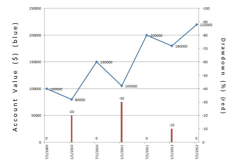
Drawdown (DD) is how much the account has lost from its all-time high. Take a look at the sample equity curve shown below:
The max DD % is -30% on 1/2/11 since the account value had fallen from $150K to $105K.
When assessing a system, it’s important to study DD because this can determine the probability of being able to trade a system consistently over the long-term. Typically, the larger the DD, the greater the Risk of Ruin, the greater the potential profit (think exponential equity curves rather than linear), and the greater the chance you will sell out at the worst time due to fear, sleepless nights, and severe anxiety when losses become largest.
Table 1 from the 9/19/12 blog post shows that when trading every 5-day period, the max DD % was -19.71% vs. -10.45% when buying the S&P 500 only when VIX is at least 5% above its 10-SMA.
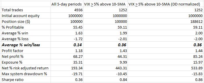
This difference, a factor of 1.88, is significant because it can be used to position size the trade. If you are comfortable with a 20% DD then you could trade the “overbought” VIX with nearly twice the position size. Column #3 from Table 1 shows system statistics using a position size of $100K * 1.88 = $188K. Note that the net % risk adjusted return increases from 443.81% to 533.89% primarily from the Exposure increase from 9.99% to 15.97%. Most other system statistics remain the same.
These results are what we should expect given my statement three paragraphs above. Position size increased by 88%. Net profit increased by 92%. The bonus is that although I adjusted position size expecting a proportional in max DD, the latter only increased by 51%. We might be able to trade this system even larger and still remain within our comfort zone.
More on position sizing at a [much] later date.
Categories: Backtesting | Comments (1) | PermalinkTrading System #1–Initial Assessment (Part 1)
Posted by Mark on September 19, 2012 at 08:37 | Last modified: September 21, 2012 06:45In my post http://www.optionfanatic.com/2012/09/14/trading-system-1-backtesting-assumptions/ (9/14/12), I discussed my assumptions for this backtest. I will now proceed with an initial assessment of the claims used to define this strategy.
This part of the system development process is my “Motion to Dismiss.” Think of me as a Defense attorney asking the judge to throw out the entire case because “it’s absurd, Your Honor.” I found these claims on the internet and the internet is often an unreliable source of information. Before I waste time developing a trading system, I want to see if the claims even have merit.
First, let’s take a look at the average 5-day return for SPY vs. 5-day return when VIX is “overbought”:
Table 1
Please ignore the third [“DD normalized”] column for the time being.
Let’s begin the analysis with total trades, net profit %, and exposure %. Realize that the “overbought” VIX condition is more restrictive than “average 5-day return,” which includes one trade beginning every single day. It’s not surprising to therefore see “all 5-day periods” having nearly four times as many trades as the other column. Exposure % measures what percentage of the account is invested during what percentage of time. Position size is fixed here at $100K but where “all 5-day periods” has open trades every day, the other column only trades when the VIX is “overbought.” At first glance, “all 5-day periods” looks impressive with a net profit % of 68.27% vs. 44.31% but don’t overlook the decreased exposure.
“Net % risk adjusted return” equates the two trades by dividing net profit % by exposure %. The result is a hypothetical simulation of both trades being completely in the market at all times. By this measure, buying only when VIX is overbought performs better than buying in general by a factor greater than two.
From a portfolio perspective, focus on the word “hypothetical” two sentences above. Net % risk adjusted return is not a realistic number. Being out of the market much of the time is the nature of the trade. It will therefore generate less profit for you. In order to realize a good profit on of your total portfolio you would need to combine this trading system with other systems to put more of your money at work more of the time.
Categories: Backtesting | Comments (3) | PermalinkTrading System #1–Brief Notes on Statistical Interpretation
Posted by Mark on September 18, 2012 at 07:24 | Last modified: September 19, 2012 06:14In addition to generating profit and loss numbers, sophisticated backtesting software will provide a whole slew of statistics each designed to address a different aspect of the performance results.
Without question, one of the most complicated matters in developing a system is how best to evaluate it. Different aspects will be more or less important to different people. One person may not care about the average win vs. average loss as long as most trades win. Another person may not care about how few trades win and how large the drawdowns get as long as net return is maximized over time. Younger people can afford to lose more because time is on their side. Retirees may be risk-averse because what they lose they don’t have so much opportunity to regain.
From a graphical point of view, many backtesting statistics describe the equity curve itself. Supposing a given initial value ($1M in our case), the equity curve shows the value of the account over time. A curve sloping up (down) is making (losing) money. Drawdowns are the difference (in dollars or percent) from an equity value peak to valley. Flat times describe time intervals between new equity highs. Most people prefer shallow drawdowns and shorter flat times to sleep easier at night. In theory, this may be achieved at the expense of total profit and exponential (sloping up more and more over time) equity curves. A lower total profit often means a safer system, however, that has a lower Risk of Ruin: probability of the account going to zero (“bust”) from a string of losses or just a couple large losses.
Like trading itself, much of system development is about tradeoffs.
Categories: System Development | Comments (0) | PermalinkTrading System #1–Backtesting Assumptions
Posted by Mark on September 14, 2012 at 05:51 | Last modified: September 21, 2012 06:42In my last http://www.optionfanatic.com/2012/09/13/trading-system-1-introduction/ (9/13/12), I provided the rationale for a system I aim to develop. The first step is to determine whether the SPX loses money (on average) when VIX has closed 5% or more below its 10-SMA and whether it gains at least twice as much when VIX has closed at least 5% above its 10-SMA.
Before proceeding with the backtest itself, let’s consider the assumptions. I assumed no slippage but an $8.00 commission charge for every trade. I assumed a starting equity of $1M and placed each trade with $100K. My maximum number of open positions was set to 5. The account equity must be large enough to avoid trade limitation and consequent distortion of results (do you understand why?). Since I’m evaluating 5-day returns and placing a trade every day, I need to allow for five concomitant trades. With a position size of $100K, the account needs to be at least $500K in size. To handle drawdowns and still allow for all trades, I arbitrarily doubled that to $1M. I could have used $10M.
Similarly, if looking at percent returns then you don’t want commissions to be a factor in the backtesting results. For this reason the initial backtest does not usually include commissions. In this case, a 1% profit per trade is $1,000. I included the commissions of $16 (round trip) because that amounts to 1.6% of the profit, which I consider negligible.
Backtesting dates are from 1/29/1993 to 8/30/2012. The former date corresponds to the first month VIX data were available.
I will continue in my next post with a brief discussion about statistical interpretation.
Categories: Backtesting | Comments (2) | PermalinkTrading System #1–Introduction
Posted by Mark on September 13, 2012 at 04:42 | Last modified: September 13, 2012 07:27The first trading system I am looking to develop is based on some material I found on the internet. The claim is that in the five days after the CBOE Volatility Index (VIX) closes 5% or more below its 10-day simple moving average (SMA), the S&P 500 index (SPX) has lost money on average. Furthermore, when the VIX closes 5% or more above its 10-SMA, SPX has outperformed the average week better than 2-1 over the next five trading days.
Can I verify these results?
The first part should be easier to backtest. I will buy at the close when VIX closes 5% or more above its 10-SMA. I will exit five days later. As a benchmark, I want to compare these results to the average 5-day period.
What seems a bit tricky about this backtest is that I will need to allow for multiple signals to be in effect at once. In other words, if VIX closes 5% above its 10-SMA today, tomorrow, and the day after, then I will need to allow for three open trades. In practice, this would be simple enough: position size to allow for a maximum of five open trades at the same time. If your account size is $100K then don’t allocate more than $20K per trade. Most backtesting software that I’ve seen will not allow for multiple trades on the same ticker triggered at different times to be open concomitantly.
Thankfully, AmiBroker does not fall prey to this restriction. AmiBroker is the market analysis software that I have struggled to learn over the past 18 months. Let’s see if I can get some answers to this first question by tomorrow.
Categories: Backtesting | Comments (1) | Permalink