Short Premium Research Dissection (Part 3)

Conclusions drawn from the table shown here are debatable.

She writes:

     > While it may be counterintuitive, selling straddles in the lowest IV range
     > was typically more successful than selling straddles in the middle-two IV
     > ranges, despite collecting less overall premium. The reason for this is
     > that when the VIX Index is extremely low, the S&P 500 is typically not
     > fluctuating very much, which leads to steady option decay that leads to

She provides no data on this, and as an EOD study, large intraday ranges may have been masked altogether. HV or ATR are better indicators for how much the market moved. IV reflects how much the market is expected to move.

     > profits for options sellers. The biggest problem with selling options in
     > low IV environments is that you collect little premium, which means your
     > breakeven points are close to the stock price.

All of this makes obvious sense. I would caution against trying to explain “the reason.” It is a reason but who knows why it is. The only thing that matters is that it was an edge in the past. Part of our job as system developers is to look deeper and see if it was a consistent and stable edge. I think it is also our job when developing systems to determine how likely the edge was to be fluke (see third paragraphs here and here), and what we should monitor going forward to know the edge persists.

Said differently, as system developers we must know what we should be monitoring in real-time to know when the system is broken. Only retrospect can ultimately determine whether a system is broken, but we must have criteria in place such that when we see something reasonably suspicious we can take action (and exit).

She continues:

     > Conversely, selling options in the highest IV range has historically
     > been successful because you collect such a significant premium, allowing
     > the market tons of room to move in either direction while remaining in
     > the range of profitability.

As before, this makes obvious sense since the data are consistent with the interpretation (reminds me of the financial media as described in the fourth-to-last paragraph here). Is this truly the reason? Not if we look back 10 years from now and see the data trends reversed.

If I were to include this content at all, I might have phrased it by saying “one way to make sense of these data is to think of low IV as… and to think of high IV as…”

Taking a step back, we do not even know if the groups are actually different without a statistical analysis (see links in the third-to-last paragraph here). And again, we do not know how many trades are in each group.

Moving onto the next table:

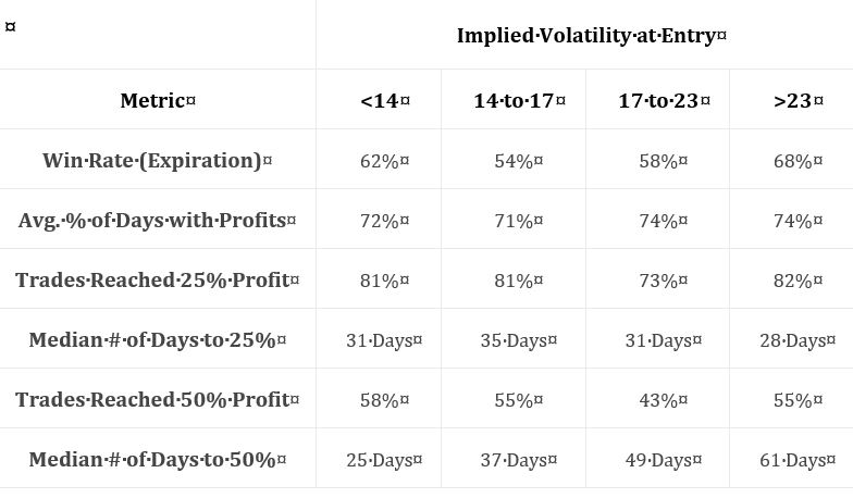
Again, no statistical analysis is performed.

However, I do think it meaningful that all groups showed 73% or more trades hitting 25% profit.

By the way, does this include winners and losers? I think it should include just winners. Do rows 4 and 6 include winners and losers? I think those should include just winners. See my last two paragraphs in Part 2 about lack of transparent methodology.

For kicks and giggles, she then writes:

     > But why do the middle-two VIX entry ranges show slightly worse trade
     > metrics compared to the lowest and highest VIX entry ranges?

At least she doesn’t try to apply the above explanations for low and high IV to these two groups!

Short Premium Research Dissection (Part 2)

I continue today with my critique of some recently-purchased research. This tells a story that should be interesting and compelling to option traders. For this reason, I don’t mind if this mini-series is lengthy.

Skipping ahead a couple sections, this table breaks down straddle data into four categories of VIX level with an equal number of occurrences in each:

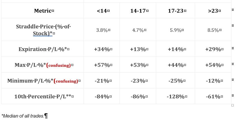
Inclusive dates and number of occurrences need to be given every time. The section mentioned in Part 1 said “since 2005” whereas text in this section says “since 2007.” Which is it?

Text in this section says “analyzing these four ranges across four different entry time frames would leave us with an overwhelming amount of data, so we’ll be using the 60-day straddles for this analysis.” I think we can therefore assume 60 DTE.* As a critique, though, I never want to see weak excuses like this when I’ve paid good money to get something. If you told me “data are condensed for simplicity” ahead of time, then I would never have trusted enough to purchase it. This screams “I’m too lazy.” The only reason to condense is for having valid reason to do so.

Row 4 is confusing because it contradicts the first table presented in Part 1 where the worst loss was stated to be -390%. These numbers aren’t anywhere close to that. Row 5, which gives the 10th %’ile to help define the distribution, is more consistent with -390%.

I miss the standard of practice for reliable methodology reporting seen in peer-reviewed scientific literature. The “methods” section of a peer-reviewed article lays out precisely-defined steps that could be followed to repeat the study. I want to see a recap of the methodology used to generate every table and graph shown in a backtesting report (see fifth paragraph here). If presented in the same section, then restatement may not be warranted. At the very least, the first table or graph in every section should be accompanied by well-defined methodology.

If I don’t even have mention of methodology to suggest the author’s head is in the game, then I have added reason to suspect sloppy and inconsistent work. Especially given the fact that people I meet in the trading community are complete strangers, I do not want to assume a thing. It’s my hard-earned money on the line and with all the stiff disclaimers up front, the author is not accountable. This is another reason why I would prefer to do my own research.

* I still want to see number of occurrences for confirmation. I want to see redundant statistics all over
   the place to cross-confirm things, really.

Short Premium Research Dissection (Part 1)

I recently purchased research from someone on short premium strategies. In this mini-series I will go through the research with a fine-tooth comb and critique it.

I am going to conduct this analysis in much the same way I have previously dissected investment presentations. Many of these offer mouthwatering conclusions. I think it’s important to smack ourselves whenever we get whiff of something sounding like the Holy Grail. We’re all looking for the Grail and we hope to find it even though, in a separate breath, experienced traders would admit no such Grail exists. Being overtaken by confirmation bias (mentioned twice in the final four paragraphs here and in the fourth paragraph here) can amount to some expensive trading tuition, indeed.

The first thing she does is present basic data on short straddles:

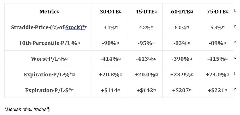
This is an interesting table. I always like to see some reference to “worst trade.” She includes 10th %’ile PnL, which is a great way of giving clues about the PnL distribution. Alone, the average (mean or median) tells very little if the distribution is not Normal. I would have liked to see more percentile data—maybe 5th %’ile (~ 2 SD) and 20-25th %’ile (~ 1st quartile)—to better define the lower tail.

Unfortunately, the methodology used to generate this table is not adequately explained. She writes “2005 to present.” When in 2005? The ending date is also unknown (the document has no publication date, either). The chart implies trades were taken every month at the specified DTE but I need to see total number of trades for verification. Anything more than 30 DTE would result in overlapping trades and much of the document discusses nonoverlapping trades. This could result in a significant sample size difference (larger sample sizes are more meaningful).

Speaking of significant differences, no statistical analysis was applied in this document. This is very unfortunate for reasons discussed here and here. Without number of occurrences and p-values, we cannot put context around whether descriptive statistics are different no matter how they appear.

This table includes more interesting exploratory data:

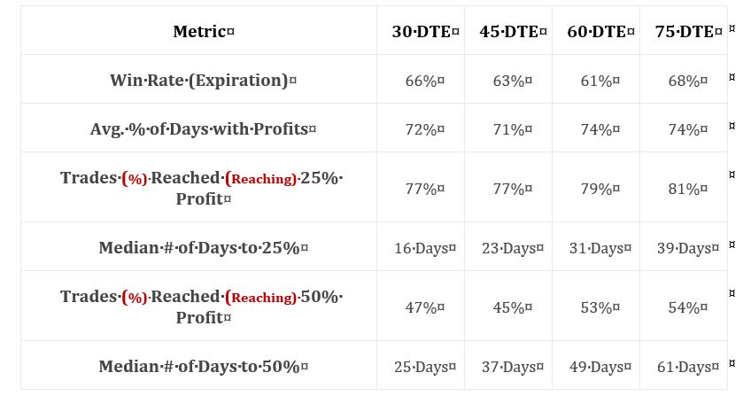
Row 1 indicates suggests a profitable trade, but whether the average trade is profitable depends on the magnitude and distribution (think histogram) of losses. Rows 3 and 5 give insight into the distribution of maximum favorable excursion (see second paragraph here), which can be used to determine profit target. Why set a 50% profit target if only 10% of trades ever reached that level? Rows 4 and 6 give temporal context, which speaks to annualized returns.

I will continue next time.

Mining for Trading Strategies (Part 3)

I continue today with two more random simulations run on short CL.

Mining 5 is a repeat of Mining 4 (results of which I covered last time) with the same minor change I made to exit criteria. Also as mentioned in Part 2, I am now running the Randomized OOS x3 for confirmation (perhaps two would be sufficient?).

Out of the top 32 (IS) strategies, four demonstrated a lower Monte Carlo (MC) analysis average drawdown (DD) than backtested DD (2007-2015). Three of the four passed Randomized OOS and none passed incubation (2015-2019).

Focusing primarily on Randomized OOS, 14 of the top 33 passed but none passed incubation. Three of the 14 are strategies that passed the MC DD criterion just mentioned.

Because this was not encouraging, I re-randomized the entry criteria, made one change to the exit criteria (see Mining 6), and ran another simulation.

Focusing primarily on the MC DD criterion, 13 out of the top 32 (IS) strategies had a lower average MC DD than backtested DD. Only four of those 13 passed Randomized OOS, and one of those four also passed incubation.

Focusing primarily on Randomized OOS, 12 of the top 32 strategies passed and four of those 12 also passed the MC DD. The only strategy in this simulation to pass incubation was one of those four.

To recap the last few posts, I have run six simulations thus far with my latest methodology. The first simulation was long. This generated six strategies that passed incubation and two that were close (PNLDD 1.70/PF 1.42 and PNLDD 1.98/PF 1.37). The last five simulations were short. Mining 3 produced two strategies that passed incubation. Mining 4 and Mining 6 produced one strategy each that passed incubation.

In other words, Mining 1 was prolific while Mining 2 through Mining 6 were relatively dry. Why might this be?

I am concerned that passing incubation is not so much a matter of whether the strategy is robust as it is a matter of whether the incubation period is favorable for the strategy. If this is true, then should incubation really be the final arbiter? I can imagine a situation where a strategy passes incubation but does not pass either of the other test periods (four years each of IS and OOS); am I to think this strategy is any better than those from my simulations that don’t pass incubation?*

Maybe number of periods passed (e.g. with PNLDD > 2.0 and PF > 1.3) is most important. With each period being slightly different in terms of market environment [whether quantifiable or not], strategies that pass more periods would seem to be most likely to do well in the future when market conditions are likely to repeat (in sufficiently general terms).

This relates back to walk-forward optimization (WFO), but remains slightly different. In WFO, I get multiple test runs by sliding the window forward the length of the OOS period. The big difference there is that the rules can change with each run. What I really want to study are rolling returns (overlapping or not is a consideration) of the same strategy and then select strategies that pass the most rolling periods. Is it possible this could happen by fluke? If so then this approach would be invalidated.

Another possibility is to seek out a fitness function that reflects equity curve consistency. I need to research whether I have this at my disposal and consider what similarities exist compared to a tally of rolling returns.

* — Realize that I don’t incubate unless the strategy does well OOS, passes Randomized
       OOS (and/or MC DD), and is reasonably good IS (else it would not have appeared in
       the first place and/or would not pass Randomized OOS per third paragraph here).

Mining for Trading Strategies (Part 2)

Today I am going to mine for more trading strategies using the same procedure presented in Part 1.

Today’s strategies will be short CL. See Mining 2 for specific simulation settings.

Seven out of the top 20 (IS) strategies passed the Randomized OOS test (see fourth paragraph here). None of the seven had a PNLDD > 1 in the 4-year incubation period, or a PF > 1.24.

Six of the top 30 had an average Monte Carlo drawdown (DD) less than backtested DD. Only two of the six passed Randomized OOS. I did not run the others through incubation.

Not happy with this, I ran another simulation (see Mining 3) for short CL strategies the very next day.

Nine out of the top 28 (IS) strategies passed Randomized OOS. With PNLDD > 2 and PF > 1.30, two of these nine passed incubation. Five of these nine had an average Monte Carlo DD < backtested DD, but none of those passed incubation. Thirteen of the top 28 strategies had an average Monte Carlo DD < backtested DD, but none of these passed incubation.

Still not impressed, I changed the exit criteria slightly for my next short CL simulation (see Mining 4).

Twenty-two of the top 31 (IS) strategies passed Randomized OOS. One of these 22 passed incubation (PNLDD 2.44, PF 1.57). Five of these 22 had an average Monte Carlo DD < backtested DD, but none of the five passed incubation.

Running this simulation generated 22 strategies that passed Randomized OOS but only one that passed incubation (and none that passed those + Monte Carlo DD). I questioned the utility of looking at so many Randomized OOS graphs since such a small percentage pass but on second thought, viewing more is necessary for exactly that reason.

I have seen strategies pass Randomized OOS once but fail to repeat. With Monte Carlo DD, I run the simulation three times for confirmation. I will do the same for Randomized OOS going forward. I also thought about requiring both OOS and IS equity curves to be all above zero for Randomized OOS. The hurdle is high enough already, though, so I will hold off on the latter and just focus on requiring multiple passing Randomized OOS results to confirm.

Mining for Trading Strategies (Part 1)

On the heels of my validation work with the Noise Test and Randomized OOS, I am going to proceed with a new methodology to develop trading systems.

I built today’s strategies in the following manner:

• Random 2-rule long CL with basic exit criteria (see Mining 1)
• Test period 2007 – 2015
• Second half of test period designated as OOS
• Strategies sorted by OOS PNLDD
• Searched on first page of simulation results for strategies that passed Randomized OOS
• Retested passing strategies from 2015 – 2019 (“incubation”)
• Looked for strategies with 4-year PNLDD > 2 and PF > 1.30 during incubation

The incubation criteria are nothing magical. I found a couple handfuls of decent-looking strategies and settled upon these numbers after seeing the first few (the numbers were actually lowered somewhat by the end). Also, more than anything else at this point I am trying to gauge whether Randomized OOS is at all helpful to screen for new strategies; a specific critical value will hopefully be determined in the future.

Of the top 28 strategies (all had PNLDD > 3.3 OOS and PF > 1.48 OOS), 21 passed Randomized OOS. Many of these satisfied DV #2 for the IS portion as well, but I did not require that in order to pass.

Nine of 21 strategies met the lowered incubation criteria with PNLDD > 1.68 and PF > 1.28.

On the Monte Carlo Analysis, I look for average drawdown (DD) to be less than the backtested strategy DD. This is mentioned by the software developers as a metric to provide confidence that performance statistics are not artificially inflated due to luck. I have not yet tested this, but I am monitoring it.

In the current simulation, zero of 10 strategies that met the lowered incubation criteria had Monte Carlo DDs less than backtested. None of the other 11 strategies that passed Randomized OOS did either.

I have no major takeaways right now since I am early in the data collection stage. What percentage of strategies pass Randomized OOS? What percentage of strategies have MC DDs less than backtested? What percentage of strategies go on to pass incubation? What kind of performance deterioration can I expect going from IS to OOS to incubation?? How often will I find a strategy that does not follow this pattern?

The software is advertised to come standard with an arsenal of tools capable of stress testing strategies. If passing those stress tests is not correlated with profitable strategies, then we will have an ugly disconnect.

For now, though, all I need are more simulations, more samples, and more data.

Testing the Randomized OOS (Part 4)

I ran into a snafu last time in trying to think through validation of Randomized OOS. Today, let’s try to get back to basics.

The argument for Randomized OOS seems strong as a test of OOS robustness for different market environments. By analyzing where the original backtest fits within the simulated distribution (DV #1), I should be able to get a sense of how fair the OOS period is and whether it contributes positively or negatively to OOS results. Also, if all simulations are above zero (DV #2) then I feel more confident this strategy is likely to be profitable during the time period studied.

In the same breath, Randomized OOS is a reflection of IS results. The better IS performance, the greater the chance for better scores on DV #1 and DV #2. I could look at the total equity curve and separately evaluate IS vs. OOS, but I think the stress test may portray this more clearly.

To make for a viable strategy, I want the actual backtested OOS equity to be in the lower 2/3 of the simulated distribution and a Yes on DV #2. I also want to see decent IS performance, but the latter is probably redundant if I am looking at Randomized OOS. My study, then, is to determine whether strategies that pass Randomized OOS are more likely to go on to produce profitable results in the future (similar to this third paragraph).

Perhaps the highest-level study I can do with the software is to build the best strategies and see what percentage proceed to do well* afterward. Since the software builds strategies based on IS results, I could save time by testing on IS and looking to see what percentage of best strategies do well OOS. This could serve as a benchmark for what percentage of best strategies that also meet stress testing criteria go on to do well. The big challenge is to find strategies that pass the stress tests. This is also the most time-consuming activity.

The latter process, though, is probably already shortened now that I have rejected the Noise Test. Related future studies include exploration of the merits of MC simulation and MC drawdown.

* — Operational definition required. “Do well” could mean positive PNL or
       some minimal score on other fitness functions.

Testing the Randomized OOS (Part 3)

Today I continue discussion of my attempt to validate the Randomized OOS stress test.

As I started scoring the OOS graphs, I quickly noticed the best (IS) strategies were associated with all simulated OOS equity curves above zero (DV #2 from Part 1). This seemed much different than my experience validating the Noise Test. I realize comparing the two is not apples-to-apples (i.e. different methodology of stress test, 100 vs. 1,000 simulations, etc.). Nevertheless, this caught my attention since only ~50% (85/167) of the Noise Tests analyzed showed the same thing.

I then realized IS performance directly affects the OOS graph in this test! The simulated OOS equity curves are a random mashup of IS equity and OOS equity. If the IS equity (or any fitness function) is really good then the simulated OOS is going to have a positive bias. If the IS equity is marginal, then it’s going to have a much weaker [but still] positive bias.

I figured my mistake was that I needed to be scoring the IS, not OOS, graphs. I would then be seeing if the best versus not-so-great strategies are associated with any significant difference in DVs #1 and #2. I realized, too, that not all IS strategies had associated OOS data that met my minimum trade number criterion (60). Were this the case, then attempting to run the Randomized OOS test produced an error message forcing me to find another strategy instead. This took more time, but I was able to get through it.

For the same reasoning described two paragraphs above, I now believe this approach to be flawed as well. My best and worst strategies are associated with an unknown variance in OOS performance. This OOS variability prevents me from establishing a direct link between any observed differences and quality of (IS) strategy. All observed differences are due to some unknown combination of IS and OOS variability.

Doing the study this way would require collection of additional data on OOS performance to compare consistency between the groups. A brief review shows 61 out of 167 (36.5%) strategies with profitable OOS periods (and I should probably go through and estimate the exact PnL to get more than nominal data). The higher the OOS PnL, the more upward bias I would expect on the IS distribution. If I have three variables—good/bad IS, not/profitable OOS, and positioning within OOS simulation—then maybe I could run a 3-way ANOVA. Three-way Chi Square? I know correlation cannot be calculated with nominal data.

Honestly, I don’t have the statistical expertise to proceed with an analysis this complex.

At this point, I’m not sure it makes sense to do the study the original way, either. If I scored the OOS graph and tried to look for some relationship with future performance, then I would need to look at IS in order to determine whether something particular about IS leaked into the OOS metrics (DV #1 and DV #2) or whether OOS metrics are the way they are due to actual strategy effectiveness. Some interaction effect seems in need of being identified and/or eliminated.

Well isn’t this just a clusterf—

I will conclude next time.

Testing the Randomized OOS (Part 2)

I described the Randomized OOS in intricate detail last time. Today I want to proceed with a method to validate Randomized OOS as a stress test.

I had some confusion in determining how to do this study. To validate the Noise Test, I preselected winning versus losing strategies as my independent variable. My dependent variables (DVs) were features the software developers suggested as [predictive] test metrics (DV #1 and DV #2 from Part 1). I ran statistical analyses on nominal data (winning or losing OOS performance, all above zero or not, Top or Mid) to identify significant relationships.

I thought the clearest way to do a similar validation of Randomized OOS would be to study a large sample size of strategies that score in various categories on DV #1 and DV #2. Statistical analysis could then be done to determine potential correlation with future performance (perhaps as defined by nominal profitability: yes or no).

This would be a more complicated study than my Noise Test validation. I would need to do subsequent testing one at a time, which would be very time consuming for 150+ strategies. I would also need to shorten the IS + OOS backtesting period (e.g. from 12 years to 8-9?) to preserve ample data for getting a reliable read on subsequent performance. I don’t believe 5-10 trades are sufficient for the latter.*

Because Randomized OOS provides similar data for IS/OOS periods, I thought an available shortcut might be to study IS and look for correlation to OOS. My first attempt involved selection of best and worst strategies and scoring the OOS graphs.

In contrast to the Noise Test validation study, two things must be understood here about “best” and “worst.” First, the software is obviously designed to build profitable strategies and it does so based on IS performance. Second, a corollary to this is that even those strategies at the bottom of the results list are still going to be winners (see fifth paragraph here to see that the worst Noise Test validation strategies were OOS losers). I still thought the absolute performance difference from top to bottom would be large enough to see significant difference in the metrics.

I will continue next time.

* — I could also vary the time periods to get a larger sample size. For example, I can backtest from
      2007-2016 and analyze 2017-2019 for performance. I can also backtest from 2010-2019 and
      analyze 2007-2009 for performance. The only stipulation is that the backtesting period be
      continuous because I cannot enter a split time interval into the software. If I shorten the
      backtesting period even further, then I would have more permutations available within the 12
      years of total data as rolling periods become available.

Testing the Randomized OOS (Part 1)

I previously blogged about validating the Noise Test on my current trading system development platform. Another such stress test is called Randomized OOS (out of sample) and today I begin discussion of a study to validate that.

While many logical ideas in Finance are marketable, I have found most to be unactionable. The process of determining whether a test has predictive value or whether a trading strategy is viable is what I call validation. If I cannot validate Randomized OOS then I don’t want to waste my time using it as part of my screening process.

The software developers have taught us a bit about the Randomized OOS in a training video. Here’s what they have to say:

• Perhaps our strategy passed the OOS portion because the OOS market environment was favorable for our strategy.
• This test randomly chunks together data until the total amount reaches the specified percentage designated for OOS.
• The strategy is then retested on the new in-sample (IS) and OOS periods to generate a simulated equity curve.
• The previous step is repeated 1,000 times.
• Note where the original backtested equity curve is positioned within the distribution [my dependent variable (DV) #1].
• Watch for cases where all OOS results are profitable [my DV #2]; this should foster more confidence that the original OOS period is truly profitable because no matter how the periods are scrambled, OOS performance will likely be positive.

I want to further explain the second bullet point. Suppose I want 40% of the data to be reserved for OOS testing. The 40% can come at the beginning or at the end. The 40% can be in the middle. I can have 20% at the beginning and 20% at the end. I can space out 10% four times intermittently throughout. I can theoretically permute the data an infinite number of times to come up with different sequences, which is how I get distributions of simulated IS and OOS equity curves.

Here are a couple examples from the software developers with the left and right graphs being IS and OOS, respectively, and the bold, blue line as the original backtested equity curve:

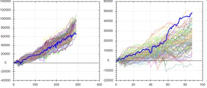
This suggests the backtested OOS performance is about as good as it could possibly be. Were the data ordered any other way, performance of the strategy would likely be worse: an ominous implication.

Contrast to this example:

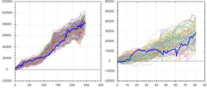
Here, backtested OOS performance falls in the middle (rather than top) of the simulated distribution. This suggests backtested OOS performance is “fair” because ~50% of the data permutations have it better while ~50% have it worse. This is considered more repeatable or robust. In the previous example, ~100% of the data permutations gave rise to worse performance.

The third possibility locates the original equity curve near the bottom of the simulated distribution.* This would occur in a case where the original OOS period is extremely unfavorable for the strategy—perhaps due to improbable bad luck. Discarding the strategy for performance reasons alone may not be the best choice in this instance.

I will continue next time.

* — I am less likely to see this because the first thing I typically do is look at
       IS + OOS equity curves and readily discard those that don’t look good.