Randomization: Not the Silver Bullet
Posted by Mark on June 17, 2016 at 06:36 | Last modified: May 29, 2021 08:53Random samples are often a research requirement but I believe trading system development requires something more.
Deborah J. Rumsey, author of Statistics for Dummies (2011), writes:
> How do you select a statistical sample in a way
> that avoids bias? The key word is random. A
> random sample is a sample selected by equal
> opportunity; that is, every possible sample of
> the same size as yours had an equal chance to
> be selected from the population. What random
> really means is that no subset of the
> population is favored in or excluded from the
> selection process.
>
> Non-random (in other words bad) samples are
> samples that were selected in such a way that
> some type of favoritism and/or automatic
> exclusion of a part of the population was
> involved, whether intentional or not.
Randomized controlled trials have been said to be the “gold standard” in biomedical research but I do not believe randomization is good enough for trading system development. Yes it would be good to avoid selection bias but this is not sufficient. I wrote about this here. The only way I can know my results are not fluke is to optimize and test the surrounding parameter space. Evaluating the surface will reveal whether a random parameter set corresponds to a spike peak or the middle of a plateau.
This perspective on randomization concurs with my last post. Perry Kaufman selected one and only one parameter set to test and for that reason I took him to task.
As Rumsey’s quote suggests, statistical bias is never a good thing. E-mail correspondence suggests Kaufman did not pick any of the values in his particular parameter set at random. He selected them based on his experience and knowledge of market tendencies. My gut response to this is “just do the work and test them all.”
While this may or may not be feasible depending on how multivariate the system, it brings to light the main objective of trading system development. I will discuss this next time.
Categories: System Development | Comments (0) | PermalinkThe Pseudoscience of Trading System Development (Part 2)
Posted by Mark on June 14, 2016 at 06:15 | Last modified: May 4, 2016 10:01Last time I outlined a trading system covered by Perry Kaufman and offered some cursory critique. Today I want to cut deeper and attack the heart of his April Modern Trader article.
With this trading system, Kaufman presents a complex, multivariate set of conditions. He includes an A-period simple moving average, a B-period stochastic indicator, a C (D) stochastic entry (exit) threshold, an E (F) threshold for annualized volatility entry (exit), and a G-period annualized volatility. Kaufman has simplified the presentation by assigning values to each of these parameters and providing results for a single parameter set:
A = 100
B = 14
C = 15
D = 60
E varies by market
F = 5%
G = 20
I believe development of a trading system is an optimization exercise. Optimizing enables me to decrease the likelihood that any acceptable results are fluke by identifying plateau regions greater than a threshold level for my dependent variable (or “subjective function“). Optimization involves searching the parameter space, which by definition cannot mean selecting just one value and testing it. This is what Kaufman has done and herein lies my principal critique.
Kaufman should have defined ranges of parameter values and tested combinations. Maybe he defines A from 50-150 by increments of five (i.e. 50, 55…145, 150), B from 8-20 by increments of two (i.e. 8, 10… 18, 20), etc. The number of total tests to run is the product of the number of possible values for each parameter. If A and B were the only parameters of the trading system then he would have 21 * 7 = 147 runs in this example. The results could be plotted.
Here is what I don’t want to see:
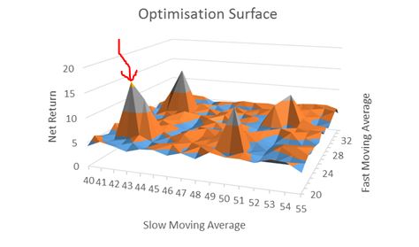
[I found this on the internet so please assume the floor to be some inadequate performance number (e.g. negative)]
A robust trading system would not perform well at particular parameter values but perform poorly with those values slightly changed. This describes a spike area as shown by the red arrow: a chance, or fluke occurrence.
Kaufman claims to have “broad profits” with his system but I cannot possibly know whether his parameter set corresponds to a spike or plateau region because he did not test any others. No matter how impressive it seems, I would never gamble on a spike region with real money. Graphically, I want to see a flat, extensive region that exceeds my performance requirements. To give myself the largest margin of safety I would then select parameter values in the middle of that plateau even if the values I choose do not correspond to the absolute best performance.
Categories: System Development | Comments (1) | PermalinkThe Pseudoscience of Trading System Development (Part 1)
Posted by Mark on June 9, 2016 at 07:11 | Last modified: May 4, 2016 08:14I subscribe to a couple financial magazines that provide good inspiration for blog posts. Today I discuss Perry Kaufman’s article “Rules for Bottom Fishers” in the April issue of Modern Trader.
In this article, Kaufman presents a relatively well-defined trading strategy. Go long when:
1. Closing price < 100-period simple moving average
2. Annualized volatility (over last 20 days) > X% (varies by market)
3. 14-period stochastic < 15
Sell to close when:
1. Annualized volatility < 5%
2. Stochastic (14) > 60
Kaufman provides performance data for 10 different markets. All 10 were profitable on a $100,000 investment from 1998 (or inception). Based on this, he claims “broad profits.” Kaufman concludes with one paragraph about the pros/cons to optimizing, which he did not do. He claims this strategy to be robust as one universal set of parameters.
In the interest of full disclosure, let me recap my history with Perry Kaufman. I have a lot of respect for Kaufman because he has been around the financial world for decades. One of the first books I read when getting serious about trading was his New Trading Systems and Methods (2005). As a bright-eyed and bushy-tailed newbie, I even e-mailed him a few questions in thinking this was truly the path to riches.
Being a bit more educated now, I see things differently.
For starters, here is some critique about what jumps off the page at me after a second read. First, four of the 10 markets are stock indices (QQQ, SPY, IWM, DIA) that I would expect extremely to be highly correlated. “Broad profits” is therefore more narrow. Second, although the trading statistics all appear decent, the sample sizes are very low. Three ETFs have fewer than 10 trades and only two have more than 50 (max 64). Finally, Kaufman provides no drawdown data. Max drawdown may define position sizing and provides good context for risk. I feel this is very important information to provide.
When I first read the article, my critique focused on a different set of ideas. I will discuss that next time.
Categories: System Development | Comments (0) | PermalinkForecasting and Accountability
Posted by Mark on June 6, 2016 at 07:15 | Last modified: April 26, 2016 09:45From an article in the April 2016 Modern Trader magazine on oil price forecasting, Garrett Baldwin wrote:
> At the heart of it is the incapability of the human mind to wrap itself
> around the sheer size and factors that go into this global market. When
> something is this large with this many moving parts, we try valiantly to
> find shortcuts or justify one specific variable. Each day, a headline
> says that oil prices fell because of whatever factor an energy journalist
> can point to that day.
>
> It’s over-simplification at best, and malpractice at worst… And it’s
> clear that no one has a clue what oil prices will hit by the end of the
> year because of so many factors beyond our grasp. No one is suggesting
> that forecasting should be abolished, but history has shown that when
> it comes to accurately predicting oil prices, all bets are off. Are we
> willing to admit we’re just not good at this?
> …
> Right now, oil prices are hovering below $30 per barrel, a level that
> was deemed impossible just a few years ago. I remember sitting in a
> lecture with a prominent economics professor not long ago. He told
> the room that we wouldn’t see oil under $100 per barrel in our
> lifetime again. He somehow still has tenure.
>
> In the end, I still argue the real problem is that there is no
> accountability. People are allowed to make any prediction they want,
> and it is quickly lost in the 24-hour news cycle. When the prediction
> doesn’t come true, the blame falls on some unforeseen variable.
The article was on oil prices but it certainly is good information to know about financial forecasting in general. Baldwin’s words are consistent with those of Bob Veras in Doomsday Forecasting (a Primer): “nobody, including those who reported your alarmist views, will check up on your track record.” The lack of accountability allows anyone to forecast anything.
Personally, I believe the fault should not fall on the forecasters but rather on the readers who try to make use of the information. Forecasting is not actionable, period. That is why I categorized this post under “financial literacy.” Once I can identify content as a forecast, I can dismiss it and move on.
Categories: Financial Literacy | Comments (1) | PermalinkLessons from David Dreman (Part 3)
Posted by Mark on June 3, 2016 at 06:42 | Last modified: April 21, 2016 07:56I want to wrap up this mini-series today on David Dreman by discussing a few more cognitive biases, or heuristics, and offering some commentary on effectiveness.
David Dreman may be a living example of a repetitive theme throughout this blog: ideas that sound good but truly have no merit. I make no performance claims about Dreman Value Management. I mentioned backtesting his idea of investing in out-of-favor issues because I have not done so myself. Contrarian investing is conventional wisdom discussed in books and seminars for traders, which is a big reason it resonates with me and feels right.
I will close with discussion of a few other types of cognitive heuristics.
Historical consistency leads to greater confidence about predictability. Dreman found investors have more confidence in a stock that consistently rises with 10% earnings growth than a more volatile stock with 15% earnings growth. Is a less volatile stock more likely to outperform into the future? That is an empirical question.
The anchoring heuristic describes a common human tendency to rely heavily on the first piece of information when making decisions. Other judgments are made in reference to the anchor, and bias exists toward interpreting other information around the anchor. For example, a stock purchase price defines what is “good” (higher subsequent prices) and “bad” (lower prices). These are purely subjective judgments. Mr. Market certainly does not care about my cost basis.
Finally, confirmation bias is the tendency to search for, remember, interpret, and favor information in a way to confirm preexisting beliefs or hypotheses while giving less consideration to alternative possibilities. The effect is stronger for deeply entrenched beliefs and emotionally charged issues, which would certainly include the prospect of making money!
Confirmation bias is the main reason I seek collaboration for trading system development, which I have written for a long time. I do not want to be blinded by confirmation bias if I get a whiff of something good. In this case, other critical minds can better maintain objectivity; the idea remains less emotionally-charged because it is not theirs.
Certainly I would rather be proven wrong in the development stage rather than with real money on the line. Confirmation bias circumvents this and collaboration is the antidote.
Categories: Wisdom | Comments (0) | PermalinkLessons from David Dreman (Part 2)
Posted by Mark on May 31, 2016 at 06:30 | Last modified: April 21, 2016 05:43David Dreman uses a contrarian investing approach in an attempt to profit from irrational heuristic thinking. Today I want to discuss Dreman’s suggestions to protect yourself from such harmful cognitive biases.
With regard to the representativeness heuristic, Dreman suggests focusing on relevant factors that may result in an entirely different investment result. Do not be blinded by similarity. Sometimes only a slight similarity is necessary to significantly resonate with us especially if a big profit/loss was realized in the previous instance.
Dreman cautions against being influenced by short-term returns of a money manager, analyst, or any kind of financial adviser. The better the numbers, the more alluring the results but this is based on an insufficiently small sample size. Look for stronger supporting evidence like a longer term track record.
Dreman suggests being doubly cautious of short-term returns when they deviate significantly from long-term averages. This applies to performance of money managers, analysts, and advisers as well as to individual stocks or funds. Mean-reversion is the rule, not the exception.
Dreman recommends patience with new investment strategies rather than expectation of quick success. Investors are more likely to adopt strategies that have recently done well, which implicates mean-reversion as an immediate headwind. One way to offset this would be to enter a strategy when it seems somewhat out-of-favor. Such a strategy has already mean-reverted or is broken altogether, in which case future outperformance will no longer result. Only in retrospect can these two possibilities be differentiated.
These are four ways to prevent biases from affecting your investing decisions.
Dreman suggests purchasing out-of-favor stocks (e.g. low price-to-earnings ratios) as one way to profit from the biases of others. While this idea sounds good, as with most other strategies I would be interested to see a large backtest to better understand context.
Categories: Wisdom | Comments (0) | PermalinkLessons from David Dreman (Part 1)
Posted by Mark on May 26, 2016 at 07:19 | Last modified: April 19, 2016 10:27David Dreman founded Dreman Value Management in 1977 and has written many books and articles on contrarian investing. In this mini-series I will highlight certain aspects of his investment philosophy that resonate strongly with me.
According to Dreman, sound investment decisions are obstructed by psychological biases that I have called heuristic thinking. Crowd behavior is therefore irrational, which leads to market bubbles and violent selloffs. Contrarian investing aims to profit from the excess.
Dreman discusses the representativeness heuristic: human tendency to draw analogies and see similarities in things that are completely different. Overemphasis on similarity leads to miscalculation if we forget to assess the actual probability of an event occurring. One example would be recognizing a company as belonging to the automotive industry and remembering what happened last time an automotive stock was purchased. Representativeness reduces perceived importance given to the variables critical in determining actual probability of the event (e.g. the stock moving higher).
Dreman discusses the law of small numbers, which is a judgmental bias that occurs when one assumes characteristics of a sample population can be estimated from a small number of observations or data points. An example would be investors flocking to the hottest mutual fund. Research suggests funds that outperform in one time period often underperform in the next. Investors also tend to follow stock analysts who have demonstrated recent accuracy rather than checking the analyst’s performance over time for a logical measure of accuracy.
Investors ignore regression to the mean. Data show a tendency for valuations and returns to revert back to long-term averages—a conclusion overlooked by investors who pile in to buy a hot stock or rush to dump out-of-favor shares.
Investors fall prey to information overload, which is related to information bias. When under siege by information, people tend to see only what they are interested in while blocking out the rest. This is related to confirmation bias. Information bias is a delusion that more information guarantees better decision making.
In the next post I will review Dreman’s recommendations to overcome heuristic thinking.
Categories: Wisdom | Comments (2) | PermalinkIs There a Better Way?
Posted by Mark on May 20, 2016 at 07:14 | Last modified: July 16, 2020 11:35This morning I take a macroscopic view wondering what I’m trying to do here and why I seem to disagree with so many others in the financial industry. It’s not just that I’m trying to find a better approach: I’m trying to determine whether a better approach even exists.
I am not exaggerating when I say almost everywhere I look, I see marketing of a better trading/investing approach (substitute “Holy Grail” to make for slight exaggeration). Many seemingly innocent, matter-of-fact claims are actually the Holy Grail in disguise but that’s beyond the scope of this post.
Just as I questioned whether successful traders exist, I question whether a better trading/investing approach exists.
Consider the following observations:
–The disappearance of popular/outspoken traders over time
–Frequent flaws in advertising/marketing claims (e.g. affirming the
consequent, hasty generalization, fallacy of the well-chosen example)
–Rampant confirmation bias
–General ignorance about trading system development and inferential
statistics: tools capable of installing meaningful objectivity into an
environment of variable moving targets
–Multiple “professionals” telling me that generation of consistent, modest
annual returns [in comparison to what many investment newsletters and
trader education programs advertise] would have the big money storming
down my door to invest if I were to start a hedge fund
–Repetitive articles in financial planning and investment periodicals about
slight outperformance relative to benchmarks translating to large AUM
—American Greed on CNBC
–Financial industry’s overall ignorance about and misrepresentation of options
to the general public
–Attraction of discretionary trading as the Holy Grail for many profit seekers
If the concept of “a better investing approach” were on trial then perhaps none of these observations taken individually would be sufficient for debunking. Taken together, however, I see a boatload of reasonable doubt.
Sometimes I feel like X-Files. On the TV program, Mulder feels compelled to continue searching to ultimately discover “the truth is out there.” With regard to finance, I wonder if there is no particular truth to be found (i.e. a better way) even though everywhere I look I see advertising suggesting there is.
Categories: About Me | Comments (0) | PermalinkBirds of a Feather
Posted by Mark on May 16, 2016 at 06:36 | Last modified: April 2, 2016 08:38“Birds of a feather flock together.” So why don’t we as retail investors? I want to spend some time discussing this based on my time spent trying to network with others and meeting with trading groups.
I have had a difficult time trying to find other traders with whom to discuss option trading much less to collaborate on trading system development. I have already written about trading as a lonely pursuit.
If I were a conspiracy theorist then I would say this happens by design. “Divide and conquer” must be an institutional mantra because working unchecked, we [retail traders] fall prey to heuristic thinking. This probably contributes in large part to the fact that 80-90% of retail traders lose money to institutional coffers.
Except I am not really a conspiracy theorist.
Varied style preferences are perhaps the biggest reason traders have difficulty hooking up. Preferences are responsible for what tickers I like to trade, what software I like to use, what time frame I like to trade, and many other considerations. Incongruity amid any of these factors may be sufficient for incompatibility. If I am lucky enough to find a trading group where 10-20 people come together then what’s the probability I will find matches across the spectrum?
Aside from individual preferences, differences in personality traits can derail a potential partnership. I may not like anger, sarcasm, conceit, or laziness. It’s almost like we need eHarmony’s 29 dimensions of compatibility to discover who will get along. This isn’t like a corporate job, either, where people are forced to cooperate or be fired. When we can walk away without obligation, we will. I have found traders (myself included) to be a very fickle lot.
Bottom line: when I overlay the low probabilities of finding an overlap in style with finding a solid personality match, it’s no surprise why the trading space ends up seeming sparsely populated. Suddenly it makes more sense why people turn to commercial means (e.g. selling newsletters, trading services, or forming “trader education” companies) in an effort to create a following and to foster community.
Categories: Networking | Comments (1) | Permalink