Curve Fitting 101 (Part 3)

Last time, I discussed how specific trade rules may result in curve fitting.

One way to avoid this is to use optimization to explore the surrounding parameter space. When applied as discussed in Part 1, optimization is a bad word. Testing all variable combinations in this manner, however, can be useful as I discussed in paragraphs 4-5 here. Borrowing from this post, look at the following visual:

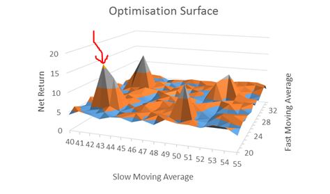
This is a three-dimensional plot with performance (net return) on the z-axis. An optimization may pick the highlighted (red arrow) peak as the best, but if it’s surrounded by losers then the results are probably more fluke (lucky) than due to signal being identified. I would feel much more confident trading a strategy in the middle of a high plateau region where I can choose variables knowing if I am a little off to either side, then I may still have a good chance for good future performance.

Do not use optimization only to choose the best; use optimization as a tool to explore the surrounding parameter space. Test all combinations and survey the landscape. Spikes are bad and high plateau regions are good. The objective is to assess the probability that good performance is not just a matter of random chance.

A standard optimization tests all variable combinations, which are called iterations. Looking back at the plot above, the iterations are ordered pairs along the xy-plane. The total iterations to be tested in a standard (exhaustive) optimization is the product of the number of values each variable can take. The Part 1 strategy had nine iterations: 20 – 100 by 10. Suppose I wanted to add an m-day exit and test exits between 3 – 21 days by an increment of three. Now I have a total of 9 * 7 = 63 iterations to test. If I also add a momentum rule and optimize momentum lookback from 10 – 30 by four, for example, then I have a total of 9 * 7 * 6 = 378 iterations. You can see how fast the iterations add up (especially if I increment by one or two instead of five or 10). This can dramatically impact computer (or especially manual: UGH!) processing time.

Going back to the Part 2 example, if I wanted to incorporate a VIX filter, then I should test different values rather than looking at just 35 (e.g. 20-50 by increments of three) to survey the surrounding parameter space.

Next time, I will discuss one final curve-fitting method.