Israelsen on Diversification (Part 3)
Posted by Mark on August 30, 2016 at 06:57 | Last modified: July 24, 2016 11:55I want to offer one further critique of Craig Israelsen’s performance data included in the last post.
As shown in the table, over 15 years the 12-asset portfolio outperformed the 7-, 4-, 2-, and 1-asset portfolio (in that order). But was this a statistically significant result?
In response to my question, Israelsen wrote:
> The issue of statistical significance pertains to
> differences among samples that are drawn from a
> population (inferential statistics). As the
> different portfolios are not samples, the issue
> of statistical difference in the returns is not
> relevant. In other words, the return of the 1-
> asset portfolio is not the mean return of that
> type of portfolio, it is THE return of that
> portfolio. Same logic for the 2-asset, 4-asset,
> and 7-asset portfolio. In essence, any
> difference in the returns is material.
I think Israelsen has a good point but I am still uneasy about his numbers. To get the returns presented, I would have to start investing on the exact same day he did. This is highly unlikely.
Alternatively, Israelsen could have created samples by studying rolling periods. This involves calculation of multiple returns over stated time intervals starting on different days. He could calculate a mean and standard deviation of all sample periods, which could then be compared using inferential statistics.
By providing one static return as Israelsen did, I believe he leaves the door open to fluke occurrence. Without knowing how likely different portfolio start dates are to dramatically affect average annual returns, no robust conclusions can be drawn. I believe Perry Kaufman made this same mistake in an article discussed recently.
I also believe Israelsen missed the point of diversification because he did not discuss drawdowns. While diversified portfolios may not result in higher annualized returns, I do believe standard deviation of returns (otherwise known as “risk”) decreases when non-correlated assets are combined.
Put another way, liked hedged portfolios I expect diversified portfolios to “lose” most of the time. This was mentioned in Part 2. However, with lower drawdowns the probability of investors holding positions through the rough times is increased. The worst outcome would be dumping the portfolio and locking in catastrophic loss from a market crash and missing a big market rebound that may be just over the horizon.
Categories: Wisdom | Comments (1) | PermalinkIsraelsen on Diversification (Part 2)
Posted by Mark on August 25, 2016 at 06:56 | Last modified: July 18, 2016 12:57Today I continue with some “words of wisdom” written by Craig Israelsen in the Feb 2016 issue of Financial Planning magazine.
> Interestingly, many investors claim to want a low-
> correlation portfolio that includes ingredients that
> do not all zig and zag at the same time. But when a
> few of their portfolio ingredients zag downward
> while other portfolio ingredients are zigging upward,
> the investor frets about the underperforming zaggers
> and becomes angry he owns a fund or stock that is
> losing money.
>
> Many investors talk the talk, saying that they want
> a low-correlation portfolio, but they can’t—or
> won’t—walk the walk and actually experience one.
As mentioned a couple times in the last post, I completely agree on an anecdotal level based on what I have heard from multiple investors during casual discussion.
Israelsen continued by providing data for different “levels of diversification” over the last 15 years. He looked at a 1-, 2-, 4-, 7-, and 12-asset portfolio. The 1-asset portfolio was 100% U.S. large-cap stocks. The 4-asset portfolio was 40% U.S. large cap, 20% U.S. small cap, 30% bonds, and 10% cash. The 12-asset portfolio was equally divided into 12 different asset classes. Annualized performance through 11/30/15:
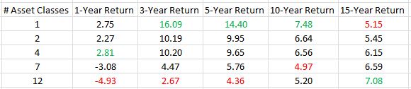
I highlighted the best (worst) performance for each column in green (red).
Israelsen writes:
> Over the three-year, five-year, and 10-year periods…
> the one-asset class investment… was the best
> performer. Finally, over the 15-year period, the
> value of a broadly diversified approach manifested
> itself with an annualized return of 7.08%…
If you’re a believer in diversification then this sounds like it took 15 years for the noise to shake out and the truth of diversified superiority to become evident.
However, from a statistical standpoint I doubt these numbers prove anything. The 12-asset portfolio performed worst over one, three, and five years. I believe one year is too short to conclude anything. 3-5 years, though? That’s at least intermediate-term. I would consider 10 years to be long-term and the 12-asset portfolio performed second worst over this interval. Given that it performed best over 15 years, I believe we have a set of performance numbers that, considered altogether, are inconclusive.
I also don’t think 15 years tells the whole story. I wonder what portfolio outperformed over 13, 14, 16, or 17 years? If it’s the 12-asset portfolio then Israelsen’s claims are substantiated. Based on the trend of numbers presented, though, I would not be surprised to see a more scattered distribution.
Israelsen writes:
> …a broadly diversified approach will lag behind
> when one particular asset class… is on a hot streak.
I don’t like this as a caveat for why the 12-asset portfolio lagged in all but the 15-year time interval. Some asset class is always going to be on a hot streak, which would suggest a broadly diversified approach will always lag. So if you want to choose a loser, make sure to diversify? That’s certainly what it can feel like and this feeds right back to the Israelsen excerpt at the top of this post.
Categories: Wisdom | Comments (1) | PermalinkIsraelsen on Diversification (Part 1)
Posted by Mark on August 22, 2016 at 06:13 | Last modified: July 16, 2016 11:07While I don’t always agree with his conclusions, I find Craig Israelsen to be a compelling contributor to Financial Planning magazine. In this blog post I address his February 2016 article “Why Not the Best?”
Israelsen writes:
> Every good planner preaches the glory of diversification…
> But here’s a reality that is less pleasant to disclose to
> a client: a diversified portfolio will never be the best
> performer in any given year…
>
> Comparing a broadly diversified portfolio with the
> best performer of the year is complete nonsense, yet many
> clients can’t resist doing it.
>
> History shows that the best performing investment in any
> year will be the stock of a company that relatively few
> people are actually invested in.
I have a couple problems with this last paragraph. First, he gives only two supporting examples. This hardly satisfies the claim that “history shows… in any year.” Two years is not every (“any”) year. Second, in order to be more rigorous he would have to define “relatively few.” Even a large cap stock, for example, has “relatively few investors” in relation to the total number of investors or certainly the total population.
From an anecdotal standpoint, I agree with this paragraph. I cannot count how many times I have heard people say “if only I had invested in XYZ” where XYZ, now significantly appreciated, traded in extremely low volume before the big run-up attracted fame and attention.
Israelsen writes:
> …every year… the best performer is always a single
> stock, never a stock mutual fund. A diversified group
> of equities can never outperform the best-performing
> single stock… for all practical purposes, the best
> return is unachievable [italics mine]…
I wholeheartedly agree.
> But here’s the rub: when we build a broadly
> diversified portfolio, it will contain some asset
> classes that do well in the current climate, and
> some that will be underachievers. That is the real
> challenge of diversifying: being patient as we watch
> the various ingredients in our portfolio take their turn
> being the hero—and the goat. If we’re not careful,
> our emotions will lead us to chase the heroes… and
> dump the goats.
Again from an anecdotal perspective, I completely agree.
I will continue with Israelsen’s article in the next post.
Categories: Wisdom | Comments (2) | PermalinkNaked Put Backtesting Methodology (Part 4)
Posted by Mark on August 19, 2016 at 07:10 | Last modified: July 15, 2016 11:26I continued last time talking about fixed notional risk. When backtesting this way, limited notional risk results in decreased granularity and significant error.
To better understand this, I listed the strikes used throughout the 15-year backtest in a spreadsheet. For each strike I calculated contract size corresponding to a defined notional risk. I then rounded and determined the error as a percentage of the calculated contract size. I started by keeping a cumulative tally of the error to see how that differed across a range of notional risk. Error may be positive or negative depending on whether the calculated contract size is rounded down or up, respectively. The cumulative tally therefore went up and down over the range of strikes and was not very helpful.
I then looked at the maximum and minimum values of cumulative error. This is what I found:
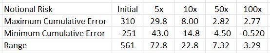
The greater the notional risk used, the lower the range of cumulative error. This illustrates the granularity issue. More granular (larger) position sizing means decreased error. Decreased error means more stability in notional risk, which I am attempting to hold constant throughout.
Backtesting my account size would have limited contract size significantly and introduced a large amount of error due to the lack of granularity. I therefore decided to increase notional risk (250x) to minimize error.
One question that remains is whether I have created an artificial situation that is incompatible with live trading. More than anything else, I am trying to get a good sense of maximum drawdown when trading this way and for this reason, I believe backtesting will provide useful information unlike any backtesting results I have seen before.
Categories: Backtesting | Comments (0) | PermalinkNaked Put Backtesting Methodology (Part 3)
Posted by Mark on August 16, 2016 at 06:40 | Last modified: July 14, 2016 11:21In my last post I described the need to keep short delta as well as notional risk constant in order to have a valid backtest throughout. Today I delve deeper into implications of maintaining constant notional risk.
Notional risk can be held relatively constant by selecting proportionate contract size. Contract size is calculated by dividing the desired (constant) notional risk by the option strike price multiplied by 100. The strike price in the denominator gets multiplied by 100 because the notional risk in the numerator has already been multiplied by 100.
Understanding the impact of rounding is important with regard to this “normalization” process. The calculated number must be rounded because fractional contracts cannot be traded. I would therefore round to the nearest whole number and this introduces error. For example, if the above calculation yields 1.3235 then I would trade one contract. One is 0.3235 less than the actual number, which represents an error of (0.3235 / 1.3235) * 100% = 24.4%. I will get back to this shortly.
My next issue was deciding what notional risk to apply. Since I was going to spend several weeks on a backtest, I decided to select a value similar to my live trading account so I could get a feel for what drawdowns I might actually see.
Trading this level of notional risk resulted in a range of contract sizes from 5 to 1. The latter is problematic because as the underlying price continues to increase into the future, the one contract would represent increasing—not fixed—notional risk. No matter how high this becomes, I cannot decrease because zero contracts is no trade.
Aside from this floor effect for contract size is a problem with granularity. By multiplying the notional risk by five, I found that over the range of strikes used in my 15-year backtest, contract sizes varied from 25 to 4. This is much less granular than the 5-to-1 seen above and would result in a much smaller error.
I will illustrate this granularity concept in the next post.
Categories: Backtesting | Comments (1) | PermalinkNaked Put Backtesting Methodology (Part 2)
Posted by Mark on August 11, 2016 at 06:41 | Last modified: June 22, 2016 15:10Last time I began to describe my naked put (NP) backtesting methodology. I thought I implemented constant position sizing—important for reasons described here—but such was not the case.
I held contract size constant and collected a constant premium for every trade. How could I have gone wrong?
The first thing I noticed was a gradual shift in moneyness of the options traded. I sold options with a constant premium. Earlier in the backtest this corresponded to deltas between 9-13. Later in the backtest this corresponded to deltas between 5-9. Pause for 30 seconds and determine whether you see a problem with this.
Do you have an answer?
The probability of profit is greater when selling smaller deltas than it is when selling larger ones. The equity curve would probably be smoother in the latter case with relatively large drawdowns. These are different trading strategies.
Even selling constant-delta options left the equity curve with an exponential feel, however. As discussed here, exponential curves do not result from fixed position size. I did notice the growing premiums collected during the course of the backtest but I thought by normalizing delta and contract size I had achieved a constant position size.
If you’re up to the challenge once again, take 30 seconds to figure out what’s wrong with this logic.
Figure it out?
The root of the problem is variable notional risk. Normalized delta and fixed contract size does not mean constant risk if strike price changes. Remembering the option multiplier of 100 for equities, a short 300 put has a gross notional risk of $30,000. Later in the backtesting sequence when the underlying has tripled in price, a short 900 put has a gross notional risk of $90,000. Returns are proportional to notional risk (e.g. return on investment is usually given as a percentage) and this explains the exponential equity curve.
So not only did I need to hold delta constant, I also needed to normalize notional risk. A constant contract size is not necessarily a constant position size. The latter is achieved by keeping notional risk constant and calculating contract size accordingly.
I will continue with this in the next post.
Categories: Backtesting | Comments (1) | PermalinkNaked Put Backtesting Methodology (Part 1)
Posted by Mark on August 8, 2016 at 06:55 | Last modified: June 22, 2016 15:34I’ve run into a buzzsaw with regard to my naked put (NP) backtesting so I want to review the development of my methodology to date.
I started with a generalized disdain for the way so much option backtesting is done regarding fixed days to expiration (DTE). Quite often I see “start trade with X DTE.” I believe this is a handicap for two reasons. First, I can only backtest one trade per month. This limits my overall sample size. Second, I don’t believe anything is special about X DTE as opposed to X + 1, X + 4, X – 5, etc. Since they should be similar, why not do them all? This is similar to exploring the surrounding parameter space and would also solve the sample size problem.
To this end, I backtested the NP trade by starting a new position on every single trading day. This is not necessarily how I would trade in real life because I might run out of capital. However, the idea was to see how the trade fares overall. This would give me over 3500 occurrences and that is a very robust sample.
From the very beginning, my aim was to keep position size fixed to ensure drawdowns were being compared in a consistent manner. In the first backtest I therefore sold a constant contract size of naked puts with defined premium (first strike priced at $3.50 or less).
This large sample size gave me a healthy set of trade statistics. I had % wins (losses). I had average win (loss) and largest win (loss: maximum drawdown). I had average days in trade (DIT) for the winners (losers). I had standard deviation (SD) of the winners (losers) and of DIT for both. I had the profit factor. I was also able to compare these statistics to a long shares position by creating a complementary shares trade over the same time interval. I then calculated the same statistics and the NP strategy seemed clearly superior.
The analysis thus far was done to study trade efficacy rather than, as mentioned above, to represent how the trade would be experienced live. To further develop the latter guidelines I would need to generate and study an equity curve. Thankfully I already had a fixed-position-size backtest so I could at least compare the drawdowns throughout the backtesting interval.
Upon further review, however, I discovered some problems that I will describe in the next post.
Categories: Backtesting | Comments (1) | PermalinkIs Option Trading Too Expensive? (Part 2)
Posted by Mark on August 5, 2016 at 06:27 | Last modified: May 25, 2016 14:59I occasionally get the sense that option trading, specifically naked put (NP) selling, is quite expensive. Today I will provide a couple other snapshots explaining why this is not the case.
Consider the purchase of 100 SPY shares at $200/share. This will cost $20,000. Suppose I sell one SPY 200 put for $2.00. This will cost me $19,800 in a retirement account. The PnL of each trade at option expiration is:
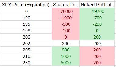
Green (red) cells indicate the more (less) profitable position. The NP trade is 1% cheaper and the naked put never loses more than the long shares. The NP underperforms to the upside but not because it loses more money—only because it doesn’t make as much. With risk traditionally defined as how much I can lose, NPs are never more risky than shares (score a second point for trading options over stock).
Are NPs too expensive? Clearly not: if I have money to buy the shares then I have money to sell the put.
I can also dramatically cut the cost of the NP by purchasing a long option. For example, in last post’s SPX example, a 1500 long put would cost $0.45. This cuts my profit from $2.13 to $1.68, which is a decrease of 22%. This cuts the trade cost, however, from $178,787 to $29,000, which is a decrease of 83%. Put another way, the potential annual return has just increased from 1.4% to 6.9%.
In the last post I discussed the possibility of selling an SPX option for 1% of the strike price to target 1% per month. The option premium increased from $2.13 to $20.75: almost 10-fold. The strike price increased from 1790 to 2010: about 13%. The former is the numerator of the ROI calculation whereas the latter is the denominator. Ponder this in terms of how much cheaper (more profitable) the trade can potentially be. Trade-offs always exist and in this case the trade-off is a decreased frequency of winning (probability of profit).
So in the final analysis, how expensive is it to trade options? Perhaps the best answer is “as expensive [or cheap] as you want it to be” (score a third point for trading options over stock).
Categories: Option Trading | Comments (0) | PermalinkIs Option Trading Too Expensive? (Part 1)
Posted by Mark on August 2, 2016 at 06:50 | Last modified: May 25, 2016 14:12My belief in trading naked puts (NP) goes back to some early posts I wrote on the topic. Occasionally, however, I am blinded by an illusion that suggests the trade is too expensive.
Consider the following SPX (S&P cash index) example. On 5/9/2016, with SPX ~2060 I could sell a Jun 1790 put for $2.13. This is 39 DTE and has roughly a 100% probability of profit based on the current implied volatility, which means its expected return is $213. This trade would cost $178,787 in a retirement account. On the same date, with SPY ~206 I could sell a Jun 200 put for $2.05. This is 40 DTE and has a roughly 82% probability of profit. This trade costs $19,795. The first trade is nine times as expensive as the second trade and potential profit for both trades is about equal!
Making matters seemingly worse is the annualized return of the initial trade: only 1.4%. If I wanted to aim for 1% per month then I could sell an option worth 1% of its strike price like the Jun 2010 put for $20.75. This has an 81% probability of profit and an expected return of $604.
[As an aside, if it were possible then buying 100 shares of long SPX would have a lousy 52% probability of profit and an expected return of negative $892. Score one point in favor of options over stock.]
At first glance above, trading the naked put did seem quite expensive but it’s less expensive in the second example.
I believe option trading is better understood as a give-and-take across different parameters. The second trade makes more money but wins less frequently. The first trade will win almost every time but make less money per trade. When the former position does lose, it may indeed be catastrophic. This is not as much the case for the latter. More (less) consistency will be met with (less) more severe, albeit rare (and more frequent), drawdowns.
I will frame this in a slightly different light next time.
Categories: Option Trading | Comments (0) | Permalink