Bullish Iron Butterflies (Part 4)

Today I continue my discussion about stratifying performance by spread width.

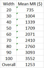
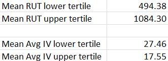
I could go one step further and adjust for margin requirement (MR), which is really net MR (spread width was gross MR; I loosely refer to either as “cost of trade”). Perhaps the 100-point trade does not actually cost five times more than the 20-point trade because more credit is received as implied volatility (IV) increases. Here are the data adjusted for MR:

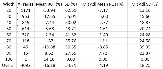
These numbers are very similar to those shown last time for spread width. This is probably because the increased IV causes a similar increase in both credit received and width:

I feel compelled to point out that this entire analysis is retrospective. I have identified the largest spread width and normalized all trades based on that value after completing the backtesting. Should I have a larger width in the future then all these results will change. This is called a “future leak” and is potentially a fatal flaw because I cannot possibly “trade like I backtest:” retrospective data is past whereas live trading is present.

Intuitively, I feel as the underlying goes higher, the cost of these butterflies and the spread widths will tend to increase. To study this, I first sorted trades by underlying price and compared the distribution of lower and upper tertiles:

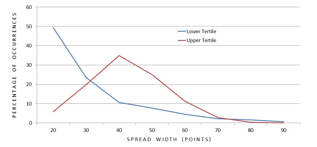
The most common width for the lower (upper) tertile was 20 (40) points. I did notice an imbalance between total trades in the groups: 1829 (880) in the lower (upper) tertile. I therefore repeated the analysis defining tertiles by number of trades:

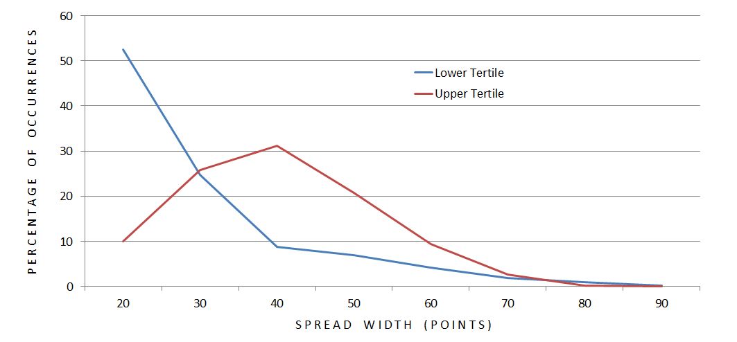
These results are pretty much the same with 1364 trades in each tertile.

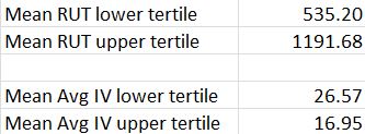
Based on this analysis I would conclude underlying price and spread width to be directly proportional. This relationship seems robust, too, since it overcomes IV trend; despite average IV being greater at lower underlying prices, the average spread width is greater at higher underlying prices.

This puts me at risk for a future trade that will cost more than those seen in backtesting. The solution is to trade these butterflies “small,” although I am a ways away from defining precisely what that means.

Bullish Iron Butterflies (Part 3)

Previous posts (here, here, and here) have led me to think I need to redo this backtest with a lowering of transaction fees from $26 to $6/contract. Because that’s going to take months, I have been deliberating over what I might be able to do beforehand to salvage the data I already have. Today I want to focus on spread width.

I have a trade-off to consider when choosing the width of a butterfly trade. The wider the butterfly, the wider the breakevens and the greater the probability of profit. The breakeven widening is less than proportional to width while the total expense (margin requirement: MR) is directly proportional, though. Why spend so much more on a wider trade to get less of an increase in breakevens? Because in terms of ROI (a percentage), I am likely to suffer a smaller loss if the market does not go my way. In other words, the market will have to move more for me to suffer 100% loss on a wide butterfly than a narrow one.

Flying under the radar of the BIBF analysis to date is the fact that I have completely left cost (spread width) out of the discussion. Despite the absence of a critical detail, the analysis appears to stands on its own: anyone disagree?

That changes today. I will stratify performance by spread width to start:

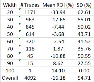
Note the dramatic ROI improvement as width increases. This corroborates the statement above that narrower butterflies are at greater risk of suffering larger percentage losses.

I have two observations to make with regard to standard deviation (SD). First, more winners and losers (on either side of zero) should contribute to larger SD. This could explain the inverse relationship between SD and spread width. Second, I would expect SD to increase with small sample sizes. While sample size (# trades) also appears to be inversely proportional to spread width, I do have acceptable sample sizes up to the 60-70-point categories. I therefore would attribute this inverse relationship more to a greater winning percentage than to higher sample sizes.

The table once again illustrates the average trade of -16%, which corresponds to the 0.44 profit factor. These numbers, reported earlier, led me to say “I do not think this is an optimistic start!”

I can eliminate spread width as a variable by taking the gross margin requirement for the widest trade (100 points * $100/point = $10,000) and allocating that for each trade. By trading this way, I am using only 20% of my capital for a 20-point ($2,000) butterfly:

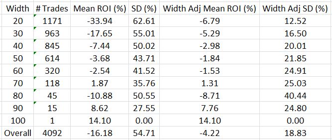
Instead of -16.18%, the average trade is now -4.22%. That is a big difference!

I will continue this discussion in the next post.

Bullish Iron Butterflies (Part 2)

With the wheels turning as a result of the last four posts (here, here, here, and here), I have decided to do an analysis of losers sorted by MFE.

I ran the analysis by simulating a reduction in transaction fees (TF) from $26/contract to either $11/contract or $6/contract. How many losers would otherwise be winners?

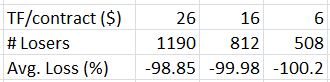
The average loss remained around 100%. The number of losses, however, decreased dramatically. Reducing TF to $11/contract and $6/contract cut the total number of losses by over 31% and over 57%, respectively.

As impressive as this may seem, the numbers are distorted because they are percentages of percentages. The losing trades are a small fraction of the whole. In order to estimate the overall impact, I counted the losers-turned-winners as +10% and adjusted the average loss downward per the numbers shown above. Here are the revised trade statistics:

For TF $6/contract, we’re now looking at a marginally (PF 1.14) profitable trade.

I believe an average loss being over seven times the average win does significant damage to the trade statistics and I can think of two ways to improve upon this going forward.

First, I can explore implementation of a stop-loss (SL). I need to look at MAE distributions of the winners to see if a SL makes sense. Winners with MAE worse than the SL will become losers and that will hurt.

Second, I can stratify performance by spread width. The statistics so far have hidden the fact that margin requirement varies dramatically across the collection of trades. Narrower butterflies have a lower probability of profit and if these amount to wasted margin then perhaps I would realize some benefit by making the narrower trades wider. Another alternative would be to trade narrower butterflies in smaller size and leave additional capital on the sidelines for dilution (e.g. a 100% loss might then be -50% although a 10% winner might then be +5%).

One important issue to address is whether I need to repeat the entire backtest with $6/contract TF’s before I proceed with the above analyses. I will sleep on that.

End-of-Day Versus Intraday Trading (Part 3)

This blog series was supposed to be complete after two posts. However, my recent discussion on transaction fees feeds right back into it so I will briefly restate some ideas with the addition of something new.

One way to effectively eliminate slippage is to enter a good ’til cancelled (GTC) closing order for the profit target. With the exception of gaps, this should take me out at +10%. What gets obscured is the fact that this order won’t usually be executed until/unless the midprice goes above +10%. For example, when the order triggers at +10% the midprice may actually be +12%. This [slippage] increases trade duration, which is similar to the negative initial PnL due to transaction fees that I discussed in the last post. The saying “time is money” has never been more true.

Trading live using a GTC order would result in a greater percentage of winners at a lower average ROI. I detailed these points in the first two parts of this blog series. To quantify how many losers might become winners, I could sort the losers by MFE; MFEs falling just short of the profit target are good candidates to become winning trades if exposed to intraday price volatility.

In terms of “something new,” I recently considered tracking the second-largest adverse excursion (SLAE). One way to analyze potential stop-loss (SL) levels is to plot MAE vs. MFE. Of all the trades with an MAE beyond a threshold level, if only a few have MFE at/above the profit target then I incur minimal risk by using that level as a SL. Many times the SL would be triggered the day before MAE is reached. Collecting SLAE data would prevent me from having to go back and retest these losers.

The problem with this idea is that trade PnL will not necessarily be SLAE when using a SL. SLAE works in a particular instance where the market is trending and a trade would be stopped out for a smaller loss the day before it would otherwise reach MAE. The SL could be triggered any number of days before MAE would be otherwise reached, though, which renders SLAE useless. Also, in choppy markets the stop-out day and MAE day may be far away in time.

SLAE is an interesting idea but not one I will add to my backtesting spreadsheet. Collecting SLAE data would take a lot of time and I can easily imagine many losers still in need of retesting with the profile of intratrade PnL being so highly variable.

Transaction Fees and Backtesting (Part 2)

My last post discussed reasons to cut back from my $26/contract transaction fee assessment. Today I want to finish up by discussing further implications of transaction fees.

A back-of-the-hand calculation suggests that if I cut transaction fees by Y then I can expect an average trade of X + Y where X was the average trade with transaction fees of $26/contract.

The relationship between transaction fees and PnL is more than linear, though. If I were to repeat the bullish iron butterfly (IBF) backtest with lower transaction fees then I could expect all the winners to remain winners. Days in trade would decrease, though, and this is the wild card.

Being in the trade for a shorter period of time reduces exposure to the IBF’s biggest enemy: big market moves. Some may argue IV spikes are the biggest enemy but the two are usually coincident.

Big market moves will damage prospects most for losing trades with highest MFE. MFE often occurs just before a big market move. In these cases, the move happens and the market never looks back thereby pushing these trades to max loss. Losing trades with MFE near the profit target have the best chance to become profitable given lower transaction fees. Confused? Consider the opposite extreme: losing trades with [lowest possible] MFE equal to initial PnL won’t have a chance regardless of transaction fees because these trades never get off the ground. For the IBF, initial PnL = -8 * transaction fees/contract.

Thought about differently, lower transaction fees means the initial PnL is greater, which means fewer days of theta decay required to reach the profit target. I could sort losing trades by MFE to approximate how many trades might benefit.

I need to make sure MFE is tracked correctly in order for this to be useful. I defined MFE as the highest intratrade PnL before expiration. I questioned this metric a couple times while backtesting. Once I suggested tracking MFE after profit target was hit could be useful. Another time I suggested tracking MFE before MAE was hit. If using stop-losses then it might be useful to know MFE before the stop-loss is hit (a better MFE afterward would be meaningless with the trade already closed).

All things considered, I think the MFE methodology is satisfactory given the need described above.

With the goal of cutting transaction fees significantly by being patient with trade entry, counting trades with MAE DTE equal to initial DTE will suggest what percentage of the time this could work. These would be the trades that recorded zero MAE (although as discussed in the last post, the opportunity would still exist to be filled intraday due to usual price volatility).

Transaction Fees and Backtesting (Part 1)

I began analyzing the data from my bullish iron butterfly (BIBF) backtest in the last post. The initial results were surprisingly poor so I want to detour and reopen the discussion about transaction fees.

Conservative assessment of transaction fees contributed to making this trade look worse than it might actually be. I also discussed this with regard to the dynamic iron butterfly. I set transaction fees to $26/contract or $208 for the whole trade. The average trade was about -$150; if I were able to do the trade for $6/contract (a nickel slippage per leg) in transaction fees then the average trade would improve to +$10. Suddenly this trade would be worth considering.

A case can be made for significantly less slippage upon exit. I spoke last time about how live trading a losing butterfly would result in significant savings: perhaps knocking transaction fees down from $104 to $30. Another example regards a profitable trade. As expiration approaches, the long legs usually decay to zero. In many cases they are worth only a nickel or dime when the profit target is hit. Rather than closing these at a cost of $26/contract, I would let them expire and save the difference.

Leaving the longs to expire also offers some end-of-cycle crash insurance were the market to make a huge move as expiration approaches. With the shorts already closed at the profit target, the longs remain risk-free. My backtesting does not take this into account. In order to see if the detail is material, I could look for big differences in maximum adverse [favorable] excursion with 2-4 DTE and the expiration PnL to get a sense of how often big moves occur in the final week.

Trade entry is another opportunity to mitigate slippage. A limit order placed at the midprice is likely to be filled within a few trading days due to the usual fluctuation in market prices. Studying MAE distribution would help to quantify this. Any trade that registers a MAE larger than -$416 is effectively a zero-slippage trade.

I am most interested to see what percentage of trades has MAE less than -$416 because these are the ones that may not fill. The risk of going unable is actually lower, though, because opportunity exists for intraday drawdowns to occur that also represent zero-slippage entries. Intraday backtesting is very time intensive so the best way to understand this is through live trading. Even if I were to use OptionVue for intraday backtesting, it only offers limited data (every 30 minutes).

Bullish Iron Butterflies (Part 1)

Today I begin my report on the bullish iron butterfly.

The structure of this trade is different from the dynamic iron butterfly. This trade was centered 2-3% above the money (split strikes were used if necessary). Also, this was a balanced (e.g. symmetrical) butterfly. The last backtest only included a few balanced butterflies [when the dynamic criterion so ordered].

Trades were held until a 10% profit target was hit on an EOD (3:30 PM ET) basis or until expiration Thursday. I assessed my usual [arguably excessive] transaction fees.

Here are the initial results:

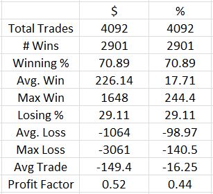
Aside from the ugly profit factor, the first thing I noticed was a max loss of -140.5%. In live trading, the worst loss I would incur on this trade would be a case where one spread goes DITM. OptionVue often shows these spreads to be worth more than their width. While this could potentially happen under low-volume, illiquid conditions, I would never actually close such a spread. Rather, I would hold it until expiration and pay two assignment fees. With this totaling $30 (or less) and the minimum margin requirement ever recorded of $400, the worst loss I could ever technically incur would be -108% ($430 / $400).

For this reason, I went back and changed the max loss on any trade to -108%:

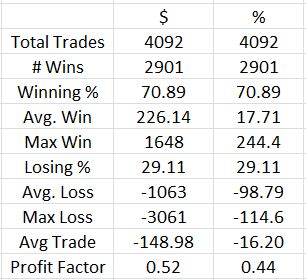
The effect of the changes was minimal. 176 additional trades showed a loss between -108% and -115% but based on the minor impact from mitigating the most extreme losses, I don’t think it’s worthwhile going back to change the others.

I’m just getting started with this backtesting analysis but I do not think this is an optimistic start! Between 2001 and 2017, I backtested the bullish iron butterfly through many market environments and conditions. While I will separate some of these out and compare in an attempt to identify differences, part of me believes a robust trade should backtest profitably on the whole. This clearly did not.