Planning My Next Meetup [hopefully not MIS] Adventure (Part 2)
Posted by Mark on July 19, 2019 at 06:58 | Last modified: January 18, 2019 09:16I previously discussed a potential Meetup model where members with sufficient expertise to present [advanced material] about option trading would have meeting/membership fees waived.
That concept, along with the rest of my thoughts from the last post, have gotten me thinking about trying to organize again. To that end, it might help to review my last attempt and why it was rejected.
I recently contacted the folks from Meetup online. I wrote the following:
> I’ve had some fits and starts with Meetup in the past so I
> want to go over my idea and see if it would be appropriate
> per your community guidelines.
>
> I want to network with serious options traders (or those
> interested to learn who would be serious about committing
> time to work together) to create a trading team where we
> consistently study simulated trades.
>
> This sort of community is badly needed. Independent traders
> like myself operate in a very isolated landscape often preyed
> upon by vendors of various types looking to profit under the
> guise of trying to help and support us.
>
> Independent traders are uncommon (most with investible assets
> hire professionals to manage their money). Option traders are
> a fraction of the fraction, which makes them even harder to
> find. I might have success in a big city like New York or
> Chicago where the trading exchanges are. In Ann Arbor, Detroit,
> or Lansing, though, I have found it to be really tough sledding.
>
> The group I envision will do most of its work online through
> something like Yahoo! Groups, Slack, or GoToMeeting. I hope
> to have daily online activity with trade monitoring and
> creation. Disciplined, consistent participation establishes
> accountability necessary to become a good trader.
>
> I would like to have a periodic in-person meeting to
> actually see and shake hands with the people we’ve been
> working with so regularly. This is where the traditional
> Meetup comes into play.
>
> Initially, I would open the group online. I would then
> like to interview each member to assess whether they are
> serious and have something to offer. I want people to
> either have expertise or time (which will eventually
> result in expertise) they can commit to studying trades.
>
> If I can find 3-10 people then I will create a virtual
> meeting of some sort to get us started. I would have
> them pay a small fee (maybe around $50) to cover Meetup
> expenses and/or anything else (including renting space
> for periodic physical Meetups down the road).
>
> Finally, I would like to focus this on the Ann Arbor,
> Lansing, and Metro Detroit area. This is bigger than a
> city: [as discussed above] I feel the need to cast a wider
> geographic net to have a real chance of finding interested
> parties. It’s all within a 90-minute driving range, though,
> which is hopefully not too large for members even at the
> extremes to make a quarterly or semi-annual
> face-to-face get-together.
>
> Any feedback would be appreciated!
I will continue with their response next time.
Categories: Networking | Comments (0) | PermalinkPlanning My Next Meetup [hopefully not MIS] Adventure (Part 1)
Posted by Mark on July 16, 2019 at 06:33 | Last modified: January 18, 2019 08:20Today I am “jotting down” some other related ideas to this blog mini-series I wrote last year.
Flashing back to the end of last year, I was aware that coming into 2018, I had some New Year’s resolutions that I aimed to fulfill. I was not happy with the progress.
With regard to work, my hope was to “get more involved” in 2018. I was thankful to have survived into my eleventh year trading full-time for a living, but I missed my pharmacy co-workers and patients (see fourth paragraph here). I had searched high and low for other full-time retail option traders but had yet to make lasting connections for a variety of reasons.
One way to become more involved would be to organize a group. As already described (in addition to link from the first paragraph, see here, here, and here), previous groups [planning] failed to bear fruit.
A different kind of group would be an educational experience for high schoolers (see third paragraph here). To this end, I reached out… but I will save this discussion for a separate post.
Here are some things that I know:
- Trading for a living is held in high esteem and described by some as the Holy Grail (e.g. trading from the beach to pay the bills without a worry in the world).
- I have searched high and low for other full-time traders with little success (e.g. fourth paragraph here).
- One trading guru opined: “people like to be spoon-fed strategies or trades. Better yet, just drop bags of cash in their lap as they sit on the couch watching TV.”
- Beginners in trading group attendance are often hoping to get free knowledge that will pay dividends.
- Most members of trading groups and forums lurk quietly without participating.
With regard to the latter, I think people who share advanced knowledge should be admitted to the group at no or minimal cost. Such a trading community currently exists. They broadcast weekly trade webinars. Anyone can attend for free, and for a monthly fee I am able to view any webinar in their entire collection on demand. If I present at one of their weekly meetings, then I get membership free for one year.
I like this model because while I believe everyone should contribute (i.e. second paragraph here), I do not wish to discriminate against beginners who are not yet able. Monetary contributions are different from sharing expertise, but they become quite important if you believe the organizer should (at least*) be partially reimbursed for expenses. Done this way, experts’ costs are covered by beginners in exchange for a sharing of experience.
I will continue next time.
* The extent to which I should be compensated as an organizer is an enticing topic for
an entirely separate blog mini-series. As discussed in the second paragraph of the
excerpt here, fees are as much for accountability as anything else. Honestly, if I knew
the next group I create would be long-lasting and hit my objectives, then I would
happily pay for it myself because my resultant trading profits would more than cover
the expense (this is a potential marketing angle, too).
Short Premium Research Dissection (Part 41)
Posted by Mark on July 11, 2019 at 06:09 | Last modified: January 15, 2019 09:57I e-mailed our author giving some general feedback about the report.
The first paragraph was the focus of my discussion from last time:
> I’ve gone over it extensively and there’s a lot I have to
> say. I don’t have solutions for some of the concerns and
> it’s possible that these particulars have no correct answers
> at all. It’s a complicated project with many permutations.
>
> I would like to see a consistent set of statistics provided
> after every single backtest. The “hypothetical portfolio
> growth” graph template is consistent. The statistics vary
> widely. I often wanted more than what you provided.
Part of this standard battery should have been PnL per day, which our author did not really discuss.
> I would also like to see complete methodology given for
> every backtest. The methodology should allow me to
> replicate your study and get the same/similar results.
>
> No explanation was given for the disappearance of
> 2007-9 data in Sct 5… It really should be in the report…
> because it could otherwise be construed as curve fitting…
> 2008 provided one of the great market shocks of all
> time and we could really benefit by seeing how the
> final trading system performed during that time.
I have since learned the data was lost because she switched from ETF to index data. The latter was only available from 2010 onward. If it meant losing 2007-9, then I think she should have stuck with the ETF.
> I wondered why some components of Scts 3-4 were not
> in Sct 5 and vice versa. How would time and delta stops
> have fared in Sct 3? How would a VIX filter and rolling
> up the put performed in Sct 5? It’s hard to compare
> Sct 5 with Scts 3-4 because of these key differences
> (along with the missing 2007-9 data).
She does not include transaction fees in the backtesting. This is a fault. I mentioned this in the second-to-last paragraph of Part 36 and the fourth paragraph of Part 38.
On several occasions (e.g. paragraph after sixth excerpt here and paragraph after first table here), I wrote “when something changes without explanation, the critical analyst should ask why.” She should be ahead of this and check herself for such inconsistencies throughout. A proofreader could help.
I have mentioned proofreading a couple times (e.g. Parts 36 and 38) and sloppiness many times in this review. Absence of that “hypothetical computer simulated performance” disclaimer was sloppy and plagued me throughout much of the report. A proofreader should have caught this.
A proofreader educated about trading system development could have flagged sloppiness suggestive of curve fitting (e.g. second paragraph below table here) and future leaks (e.g. this footnote and third paragraph below last excerpt here).
Sample sizes should always be given and the report (e.g. third paragraph below third excerpt here and first bullet point below table here) would be better with inferential statistics [testing] to identify the real differences (e.g. third paragraph below first table here and second paragraph below final excerpt here). Criteria for adopting trade guidelines should be detailed at the top. Control group performance would also be useful (e.g. paragraph below graph here and third paragraph following table here).
In conclusion, I think the report would be better described as a trading strategy than a fully developed system. With regard to the latter, though, the report is a great educational piece and a valuable springboard for further discussion.
Categories: System Development | Comments (0) | PermalinkShort Premium Research Dissection (Part 40)
Posted by Mark on July 8, 2019 at 07:14 | Last modified: January 11, 2019 09:18By way of recap, let’s begin by doing an updated parameter check (see second paragraph here). Get your reading glasses:
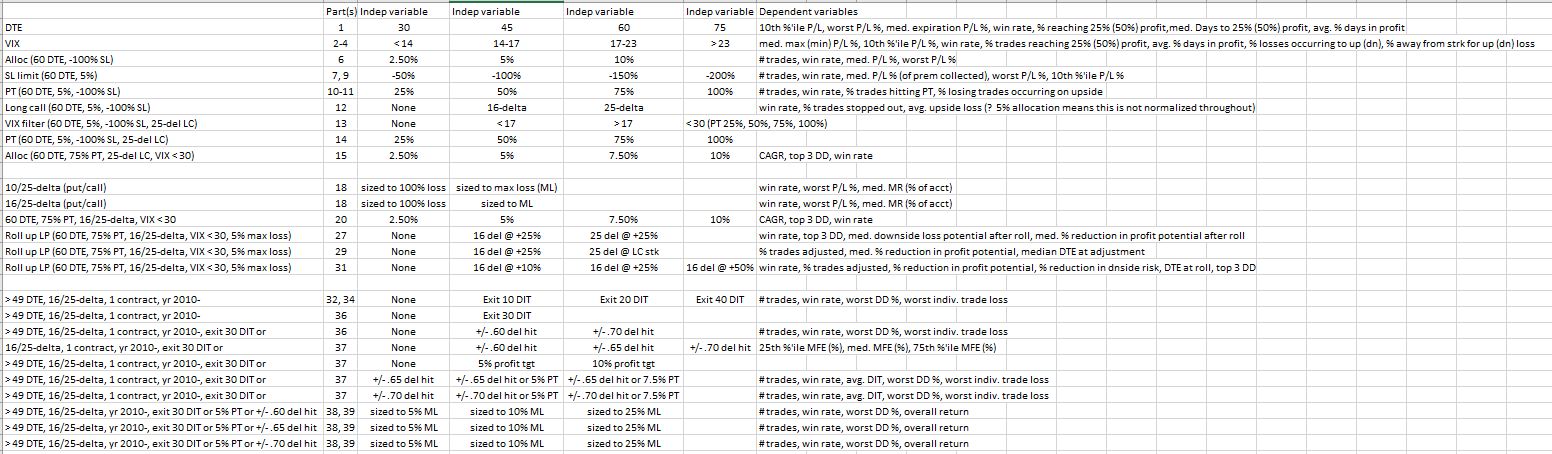
The second column shows in what part of this blog mini-series each study is discussed.
This is too complex to be a definitive exercise in trading system development. Numerous independent variables, dependent variables, and criteria of all sorts have been covered. With all the degrees of freedom represented, only a fraction of the total number of permutations are actually explored.
I discussed my concept of trading system development in the paragraphs #2 and #3 below the excerpt here. As mentioned in the second and third paragraphs of Part 11, thousands of different permutations is too complex. The scary thing is that in some instances (e.g. paragraph after graph here and paragraph #2 here where I discussed failure to explore range extremes), I have actually been clamoring for more parameter values to be studied.
I believe each independent variable should be studied separately to understand its impact on performance.* “Independent variable” is easily confused with words like entry/exit criteria, profit target, filters, stops—when in fact they all probably represent degrees of freedom. The total number of permutations is multiplicative across the number of potential values for each independent variable. I tracked this earlier (final sentence of Part 11) before the research went in too many directions with too many inconsistencies and too much sloppiness.
Some of the tested variables are more about position sizing than trade setup. I’m talking about delta selection for long options. Narrower spreads carry lower margin requirements and allow for greater leverage (see discussion beginning here). This makes delta a factor in position sizing, which goes hand-in-hand with allocation: something she does study.
An entire knowledge domain exists to solve the problem of optimization. I have yet to write about this subject.
For now, it will suffice to say that although I think our author has failed to undertake a valid system development process, I do not have the solution to right her ship. The approach seems too multi-dimensional. In my gut, I sometimes feel that not everything needs to be thoroughly explored. For example, why not just stick with 60 DTE rather than having to look at 30, 45, and 75 DTE? This is precisely the rationale for studying daily trades (second-to-last paragraph here), though, as a check to ensure results aren’t fluke. It’s really all about cutting through the laziness.
I will conclude next time.
* This is easier said than done as interaction effects (see this footnote) should also be identified.
Categories: System Development | Comments (0) | PermalinkShort Premium Research Dissection (Part 39)
Posted by Mark on July 5, 2019 at 07:03 | Last modified: January 11, 2019 08:33Continuing on with our author’s final analysis, she presents two “hypothetical portfolio growth” graphs for each of three delta stops: one with curves for 5% and 10% allocation and one with a curve for 25% allocation. Y-axis values and derived percentages are therefore relevant (see second-to-last paragraph here). None of these final graphs has a referent for the asterisk,* which we now know corresponds to the “hypothetical computer simulated performance” disclaimer shown here.
For each delta stop, she provides the usual table that falls short of the standard battery (second paragraph):
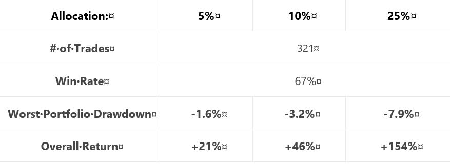
Similar to tables included previously (e.g. Part 15 and Part 20), a couple differences are noteworthy. First, she includes only the biggest rather than top 3 drawdowns (discussed in paragraph #2 below excerpt #1 here). This is characteristic of all tables in this final section (along with the lost 2007-2009 data, which was discussed in these final three paragraphs).
The other difference is inclusion of overall return rather than CAGR. As described in the paragraph below the first table here, things are sloppy when inconsistent from one sub-section to the next. This is the first time we are seeing “overall return.” Also as discussed in that same paragraph, the critical analyst should ask “why” when something changes without explanation. It’s no big deal here either, though. While overall return impresses more (larger in magnitude), CAGR works fine.
I have been calculating CAGR/MDD throughout this mini-series (e.g. Parts 33, 25, 22, 21, 20, 15). To convert from overall return, I’d have to approximate the backtesting interval (she never gives us the exact dates). I could then calculate CAGR/MDD, although it would not be comparable to previous sections due to the unexplained lost data.
Another source of significant sloppiness is passive disappearance of the VIX filter. The VIX filter was used in generating the final graph of the previous section (shown here). Like the lost data, the VIX filter has been absent in these “most up-to-date trading rules.” If the filter only comes into play for the 2008 crash, then it may represent curve fitting. Some explanation should be given for its sudden omission to preserve our author’s credibility.
With regard to sizing this strategy per individual risk tolerance, she unfortunately does not backtest an expanded parameter range (Part 38, paragraph #2) to help us truly understand allocation limits.
In the final sub-section, she presents a recent trade that probably serves a marketing purpose more than anything else. It’s always nice to hit the profit target after only five days. Beginning November 2, 2018, it probably was not included in the historical backtesting, which is fine (less fine is the omission of backtesting dates). I think something current stokes confidence more than something stale. I often wonder how many people click to order reports, trading systems, trader education products, etc., from websites with content a few years old at best. The graphs always look good. Only when you look close and dig deeper are you well-poised to identify errors and expose the fiction.
I will begin to wrap things up next time.
* The rare +1 she scored in Part 38 paragraph #4 is effectively offset.
Short Premium Research Dissection (Part 38)
Posted by Mark on July 2, 2019 at 07:22 | Last modified: January 8, 2019 06:42In paragraph #2 below the first table, I said I liked our author’s exploratory backtest to assess the [MFE] distribution.
What I don’t like about this approach is a failure to explore the extremes. I mentioned this in the paragraph after the graph here. Backtesting over a range where results are directly proportional is of limited utility. Backtesting over an expanded range can illustrate floor and ceiling effects, which defines the profitable range. With regard to delta stops (profit target), I would have liked to see 0.60 (2.5%) along with 0.75 – 0.80 (10% – 15%) rather than just 0.65 and 0.70 (5% and 7.5%).
Not only is study of the extremes* useful, I can argue for it to be essential. Exploring the tails can help us understand whether we have a normal, thin-, or fat-tailed distribution. I could imagine our author giving the excuse she wanted to avoid “overwhelming” us with lots of excess data (second paragraph below table here). It’s not excessive, though, and without it we have no reason to think she actually checked it herself. Not checking would be sloppy, superficial research indeed.
In the next sub-section, our author discusses trade sizing and the commission benefits of index vs. ETF trading. Once again (as discussed near the end of Part 36), she promotes a brokerage, which signifies a clear conflict of interest. Discussing commissions but not slippage is, if you think about it, very sloppy. These are the two biggest components of transaction fees, but slippage likely dwarfs commissions. The only place slippage is even mentioned is the “hypothetical computer simulated performance” disclaimer shown here and included in all such graphs this section (+1 on consistency, for once).
The next sub-section is titled “final strategy backtests… with various allocations.” Are we now going to see what trade guidelines have made the final cut?!
No.
She proceeds by showing us “hypothetical performance growth” graphs and cursory trade statistics for a 5% profit target managed at 30 DIT or delta stops of 0.60, 0.65, or 0.70 with allocations of 5%, 10%, or 25%. She then tells us to decide based on our own individual risk (drawdown) tolerance.
For each of the three delta stops, she gives the following [incomplete] methodology:
> Expiration: standard monthly cycle closest to 60 (no less than 50) DTE
> Entry: day after previous trade closed
> Sizing: 5%, 10%, 20% Allocations [emphasis mine]
This is a typographical error: 20% should be 25%. As with the first paragraph below the first excerpt of Part 36, maybe the proofreader fell asleep? Sloppiness has been a recurrent theme throughout.
> Management: exit after 30 days, 5% profit, or at ±0.60 short delta
I will continue next time.
* Incidentally, backtesting over an expanded range would preclude the need for an exploratory
test to determine MFE distribution.
Short Premium Research Dissection (Part 37)
Posted by Mark on June 27, 2019 at 07:02 | Last modified: January 8, 2019 05:53In this “most up-to-date” section (see end Part 31), our author has explored time stops, delta stops, and now profit targets.
As a prelude to determine what profit targets are suitable for backtesting, she gives us this table:
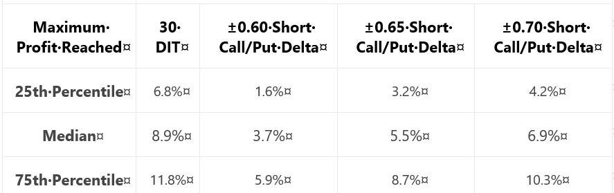
Recall from the end of Part 35 that when something changes without explanation, the critical analyst should ask why. She did not include the 0.65-delta stop last time: why? In this case, it’s no big deal. I like backtesting over a parameter range and having three values across the range is better than two. If only for the sake of consistency, I would have liked to see 0.65 data both times because it feels sloppy when things change from one sub-section to the next.
Adding to the sloppiness, she is once again lacking in methodology detail. I like the idea of probing the distribution to better understand where profit might land. If we can’t replicate, though, then it didn’t happen. Did she backtest:
- Daily trades?
- Non-overlapping trades?
- Winners?
- Winners and losers?
- Any [combinations] of the above?
These factors can all shape our expectations for sample size (which determines how robust the findings may be) and magnitude of averages (e.g. winners will have a higher average max profit than winners and losers. See Part 24 calculations).
She writes:
> Based on the above table, it appears profit targets
> between 5-10% seem reasonable to test for all of the
> approaches except the ±0.60 delta-based trade exits.
She then proceeds to give us “hypothetical portfolio growth” graph #17 with [hypothetical computer simulated performance disclaimer and] 30 DIT, 5% profit target or 30 DIT, and 10% profit target or 30 DIT.
Next, she gives us a “hypothetical portfolio growth” graph and table each for 0.65- and 0.70-delta stops. The graphs are all similar with no allocation, no inferential statistics, and nebulous profitability differences. The tables take the following format:
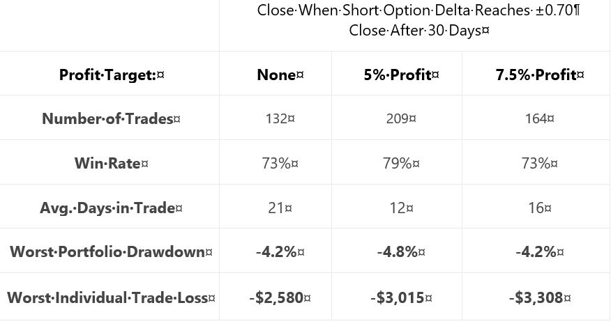
This falls far short of the standard battery and also lacks a complement of daily trade backtesting (see fourth-to-last paragraph here). We still don’t know her criteria for adopting trade guidelines, either. I therefore like her [non-]conclusion:
> After analyzing the various approaches and management
> levels, it seems you could pick any one of the variations
> and run with it. Consistency seems to be more important
> than the specific numbers used to trigger your exits.
She also writes:
> Interestingly, not using a profit target with the ±0.70
> delta-based exit was the ‘optimal’ approach historically.
For this reason and because she did not test [all permutations of] each condition[s], I remain uncertain whether a delta stop is better than any or no time stop. I would say the same about profit target: too much sloppiness and too few methodological details [and transaction fees as discussed at the end of Part 36] to know whether it should make the final cut.
I will continue next time.
Categories: System Development | Comments (0) | PermalinkShort Premium Research Dissection (Part 36)
Posted by Mark on June 24, 2019 at 07:10 | Last modified: January 2, 2019 11:17Picking up right where we left off, our author gives the following [partial] methodology for her next study:
> Expiration: standard monthly cycle closest to 60 (no less than 50) DTE
> Entry: day after previous trade closed
> Sizing: one contract
> Management 1: Hold to expiration
> Management 2: Exit after 30 days in trade (10 DIT)
I think this should be “30 DIT.” The proofreader fell asleep (like third-to-last paragraph here).
Here is “hypothetical portfolio growth graph” #15:
The two curves look different; a [inferential] statistical test would be necessary to quantify this.
She concludes the time stop results in smoother performance and smaller drawdowns. Once again, I’d like this quantified (e.g. the standard battery). I’d also like a backtest of daily trades (rather than non-overlapping) for more robust statistics.
Next, she adds delta stops:
> Management 1: Hold for 30 days (30 DIT)
> Management 2: Exit when short call delta hits +0.60 OR the short put delta hits -0.60
> Management 3: Exit when short call delta hits +0.70 OR the short put delta hits -0.70
I like the idea of a downside stop, but I question the upside stop. With an embedded PCS, we are already protected from heavy upside losses. She does not test downside stop only.
Here is “hypothetical portfolio growth” graph #16:
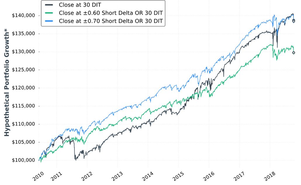
The blue curve finishes at the top and is ahead throughout. The black curve finishes on top of the green, but only leads the green for roughly half the time. Inferential statistics would help to identify real differences.
Thankfully, each of the last two graphs are presented with that “hypothetical computer simulated performance” disclaimer (see second paragraph below graph in Part 34).
Here are selected statistics for graph #16:
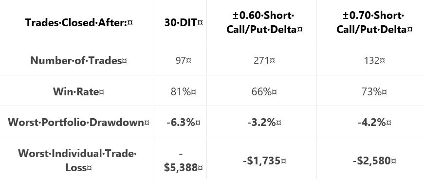
As discussed in the second-to-last paragraph here, percentages are not useful on a graph without allocation. I think relative percentages can be compared, however, when derived on the same allocation-less backdrop.
Unfortunately, we have no context with which to compare total return. As mentioned above, we’re lacking the standard battery (second paragraph) and complement of statistics for daily trades.
As with Part 34, other glaring table omissions include average DIT (to understand impact of delta stops), and PnL per day.
Transaction fees (TF) could adversely affect the delta-stop groups because they include more trades. Our author now mentions fees for the first time:
> …many more trades are made… [with] delta-based exit… we need to
> be considerate of commissions… [At] $1/contract, the ±0.60 delta exit
> would… [generate] $2,168 commissions… if you trade with tastyworks,
> the commission-impact of the strategy could be substantially less…
Unfortunately, she mentions fees only to give a brokerage commercial. Her affiliation with the brokerage is clear because she offers the research report free if you open an account with them. In and of itself, this conflict of interest would constitute a fatal flaw for some.
Discussing commissions but not slippage is sloppy and suspect. It is sloppy because as a percentage of total TF, slippage is much larger than commissions. It is suspect because neither is factored into the backtesting, which makes results look deceptively good.
Thus ends another sub-section with nothing definitive accomplished. She may or may not include time- or delta-based stops in the final system and if she does, then she has once again failed to provide any conclusive backing for either (also see third paragraph below first excerpt here).
Categories: System Development | Comments (0) | PermalinkShort Premium Research Dissection (Part 35)
Posted by Mark on June 21, 2019 at 07:37 | Last modified: January 3, 2019 06:54Finishing up the sub-section from Part 34, our author writes:
> At the very least, when incorporating short premium options
> strategies… it may be wise to implement time-based exits
> to avoid large/complete losses and reduce portfolio volatility.
By not stating definitive criteria, she [again] tells us nothing conclusive. As discussed in the second paragraph after the first excerpt here, we’ll have to wait to see if a time stop makes the final cut.
Unlike the 50% profit trigger for rolling puts to 16 delta, I think the time stop is beneficial. I wish she had shown us the top 3 drawdowns as done previously (e.g. Part 31 table). Seeing improvement on each of the top 3 would be stronger support for time stops than improvement on just the worst. Even better would be the entire standard battery (second paragraph).
Unfortunately, we do not know how time stops would impact the high-risk strategy, which was backtested before 2018.
I can’t help but wonder why time stops were not studied before 2018 (final excerpt Part 31). Admittedly, I would have suspected curve fitting had she written “due to the horrific drawdown suffered in Feb 2018, I tried to add some conditions to make the strategy more sustainable.” Not giving any explanation makes me suspect the same. I think the best approach to avoid being influenced by disappointing results is to plan the complete research strategy in advance (second paragraph below excerpt here). Exploring the surrounding parameter space (see second paragraph here) is critical as well.
> The next trade management tactic we’re going to explore
> is the idea of ‘delta-based’ exits.
Like time stops, this is another completely new idea for her. As just discussed, this ad hoc style bolsters my suspicion (see third paragraph below excerpt in Part 30) that she spontaneously tosses out ideas with the hope of finding one that works. Given enough tests, success by chance alone is inevitable. “Making it up as we go along” to cover for inadequate performance is a flawed approach to system development.
> To verify the validity of using delta-based exits, let’s look
> at some backtests to compare holding to expiration, adding
> a time-based exit, and then adding a delta-based exit.
Layering conditions is confusing because order may matter* and all permutations are not explored (see second and third paragraphs here). For example, she does not study a delta-based exit without a time-based exit. I would rather see each condition tested independently with those meeting a predetermined performance requirement making the final cut.
> First, let’s compare… holding to expiration… [with]…
> exiting after 30 DIT.
Where did 30 come from? The exploratory studies (Part 34) looked at 10, 20, and 40 DIT.
When something changes without explanation, the critical analyst should ask why. This is becoming a recurring theme (as mentioned hear the end of Parts 32 and 33).
I will continue next time.
* In statistics, this is called interaction.
Short Premium Research Dissection (Part 34)
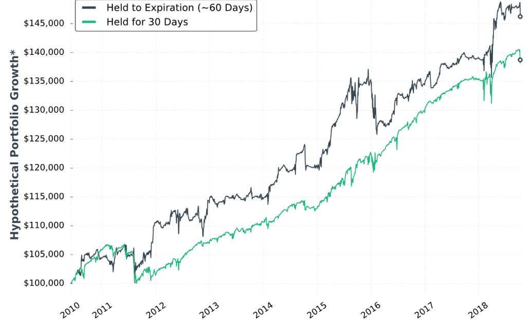
Posted by Mark on June 18, 2019 at 07:00 | Last modified: December 31, 2018 13:29Continuing with exploration of time stops, our author gives us hypothetical portfolio growth graph #15:
As discussed last time, this is based on one contract traded throughout. The hypothetical portfolio is set to begin with $100,000. This is fixed-contract position sizing. One consequence of fixed-contract versus fixed-risk (fractional) is a more linear equity curve rather than exponential. As discussed [here], the latter reaches higher and looks more appealing despite having greater risk. I have traditionally been a proponent of omitting position sizing from backtesting to allow for what I thought would be apples-to-apples comparison of drawdowns throughout (see here). In these graphs without any allocation, position sizing is effectively eliminated from the equation.
Accompanying the graph is that disclaimer about hypothetical computer simulated performance. This was a big deal earlier in the mini-series when I discussed the asterisk following the y-axis title “hypothetical portfolio growth” (second paragraph here). The disclaimer appeared for the first time in Part 16 and alleviated many pages of confusion. After that, the disclaimer disappeared leaving the asterisk without a referent until the two most recent graphs.
Score a point for completeness—however transient it may be—rather than footnote false alarm and sloppiness.
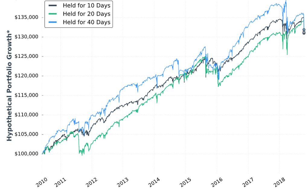
I can’t discern much with regard to differences on this graph. Final equity is ~$130,000 for all. 40 DIT > 10 DTE > 20 DTE for most of the backtesting interval, which suggests these differences might be significant were inferential statistics to be run.
She gives us the following table:
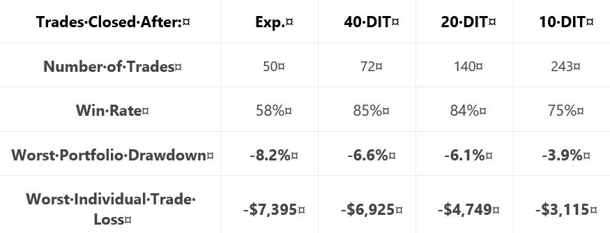
This is not the first time she tells us number of trades, but she falls far short of reporting it every time. Number of trades range from 50 – 243 over roughly eight years. That is ~6 – 30 trades per year or ~0.5 – 2.5 trades per month. On their own, these aren’t tiny samples. Backtesting one starting every trading day (e.g. second paragraph below graph here), though, would give a sample size in the thousands. I think that would be a useful complement to what we have here.
Glaring omissions in this table include average DIT (for the expiration group), total return or CAGR, and PnL per day. A big reason for using a time stop is to improve profitability (either gross or per day): show us! Time stops aim to exit trades earlier: show us [how long they run otherwise]! Nothing is conclusive without these.
Another big shortfall is the exclusion of transaction fees. Number of trades varies 2-5x across groups. The fees could add up.
I would still like to see that lost data [discussed last time] back to 2007.
On the positive side, the table does a decent job of showing performance improvement with max DD and max loss if we assume equal total return as suggested in the graph.
Categories: System Development | Comments (0) | Permalink