Trading System #2–Consecutive Directional Close (Part 4)
Posted by Mark on November 7, 2012 at 07:14 | Last modified: October 30, 2012 09:45In http://www.optionfanatic.com/2012/11/06/trading-system-2-consecutive-directional-close-part-3, I began to analyze what turned out to be some confusing data. Today I will try to better sort this out and see if the Consecutive Directional Close (CDC) trading system is one to salvage or discard.
To refresh your memory, you may look back at Figure 1 and Table 2 from the last post. Here is a slightly different snapshot reflecting what I found:
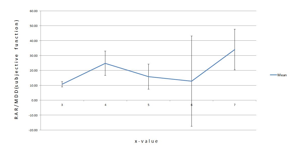
Figure 1
This graph shows the mean RAR/MDD for x ranging from 3 to 7. To establish an x-value as “best,” one point must be separated above the others with no overlapping error bars. Because of the large error bars (especially on x = 6), no points show separation.
Are there any statisticians in the crowd? What is going on here?
This is a problem with sample size:
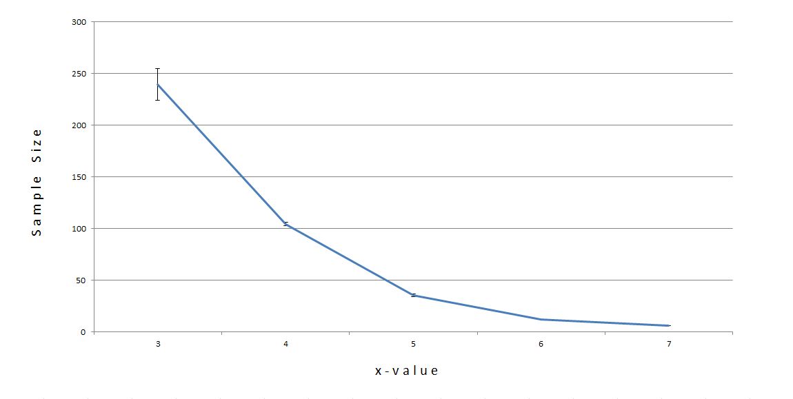
Figure 2
The number of trades for x = 5, x = 6, and x = 7 were about 35, 12, and 6 respectively. Those numbers are too small for a valid sample size. I was not overjoyed with 57 trades in http://www.optionfanatic.com/2012/10/25/trading-system-1-spy-vix-part-9 but anything under 50 is totally unacceptable.
I must do something to increase the sample size from which to draw conclusions that may be predictive of future trading. To this end, I have two ideas. First, I can backtest other broad based indices and combine the results of all trades. Second, I can backtest the basket of 500 stocks that constitute the S&P 500 (SPY) separately. Although this may create more problems than it might solve, it can certainly be instructive for me to pursue.
I will continue with this analysis in my next post.
Categories: Backtesting | Comments (1) | PermalinkTrading System #2–Consecutive Directional Close (Part 3)
Posted by Mark on November 6, 2012 at 05:41 | Last modified: October 25, 2012 15:24In my last two posts, I talked about redundant trade signals. At this point I am going to ignore redundant signals to get a feel for how the Consecutive Directional Close (CDC) trading system performs all by itself.
I began backtesting in http://www.optionfanatic.com/2012/11/01/trading-system-2-consecutive-directional-close-part-2 by studying x=3 and n=5. Now, I’m going to run an optimization to get a sense for backtesting results for x and n ranging between 3-7 (25 total systems). Just because I have another month of data, I’m going to extend the backtesting period to 9/30/2012:
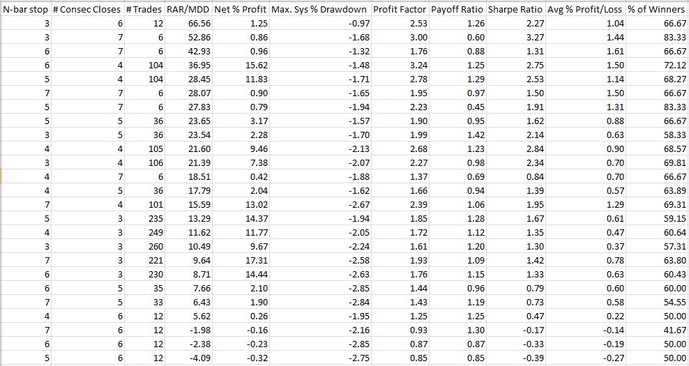
Table 1
In contrast to http://www.optionfanatic.com/2012/10/02/trading-system-1-spy-vix-part-3-2, the first thing I notice here is that only 88% of these backtested systems were profitable. While 22 out of 25 is a high number, it falls short of the 100% I saw with the SPY VIX trading system.
The next thing I notice are some inconsistencies across x. This is a mean-reversion trading system and I would expect that more CDCs would result in larger returns. Indeed, the top three systems all had six or seven CDCs. However, the four worst-performing systems (including all three losers) also had six CDCs.
If I graph these numbers to check for plateau regions:

Figure 1
This is a much different graph than Figure 1 in http://www.optionfanatic.com/2012/10/11/the-subjective-function-part-5 where with a couple minor exceptions, the curve representing the most (least) extended trade condition was on top (bottom). Here, x = 6 starts out on top and dives into negative territory. x = 7 or x = 4 (can’t tell which) is below that followed by x = 5 and, as expected, x = 3 on the bottom (not really).
When I averaged across n-values, the statistics support the inconsistency:
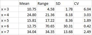
Table 2
The huge range for x = 6 is seen here as it went from the best performing system to losing money. With higher CV (large mean and small SD) favorable, x = 3 looks impressive but its mean RAR/MDD is smallest and not very impressive.
I will continue this analysis with my next post.
Categories: Backtesting | Comments (2) | PermalinkRedundant Trade Signals (Part 2)
Posted by Mark on November 5, 2012 at 04:40 | Last modified: October 24, 2012 11:40I have been discussing the implications of allowing redundant signals to trigger additional positions once already in a trade. In http://www.optionfanatic.com/2012/11/02/redundant-trade-signals-part-1, I presented results for x=3 and n=5 with redundant signals allowed and compared this to results in Table 1 from http://www.optionfanatic.com/2012/11/01/trading-system-2-consecutive-directional-close-part-2. I’d like to conclude this discussion with a point about position sizing.
Taking additional trades with multiple signals makes the position sizing consideration much more difficult. Before, no more than $100K of risk would ever be present. With multiple signals, however, up to five positions may be open. Am I comfortable with up to $500K of risk being on the table or do I need to decrease position size? With greater risk, it makes sense that greater reward (net profit %) and greater DD could both be incurred. Perhaps max DD is still the best proxy for risk and what position size should be based on.
Performance calculations are also more difficult with multiple open positions. If you are able to trade five open positions at once then returns must be calculated on $500K (in the denominator) whether or not five positions were open during that time period. The capital must be ready to be deployed if it is needed.
Considerations about position size and redundant signals are examples of what make system development so difficult. Trying to balance profit potential with risk and exposure with position size can truly be a mind-boggling experience. I sometimes feel like I am chasing my own tail! Ultimately, I will stick with the subjective function (RAR/MDD) to choose the system for me and then position size from there. Every trader needs to do the same thing tailored to his/her own preferences.
In my next post I will continue analysis of the Consecutive Directional Close trading system.
Categories: System Development | Comments (0) | PermalinkRedundant Trade Signals (Part 1)
Posted by Mark on November 2, 2012 at 06:06 | Last modified: October 24, 2012 11:27In http://www.optionfanatic.com/2012/11/01/trading-system-2-consecutive-directional-close-part-2, I presented some initial results for the Consecutive Directional Close trading system with x=3 and n=5. Today I will continue discussion of overlooking redundant trade signals.
Redundant trade signals are buy or sell signals that occur once a trade is already open. They may be in the same or opposite direction as the original trade and they may be taken or ignored.
From a statistical perspective, I always wonder whether taking just the first signal in backtesting is biasing the results. If the system backtests profitably and I only took first signals then who isn’t to say in the future, results from the first signal wouldn’t be results from the second, third, or any other signal that may not be profitable? By taking all trades into consideration I might eliminate this bias.
On another hand, results from redundant signals might not be independent of each other. In case of a mean-reversion trading system where redundant signals represent greater and greater stretching of a rubber band likely to snap back to resting state, I would expect additional trades to be more profitable. To backtest only the first signal would therefore understate the results. This would be acceptable because if a backtested system looks good to me when understated then I feel more confident it will do well when traded live.
In contrast to Table 1 from my last post, here are the results with x=3 and n=5 when redundant signals are taken:
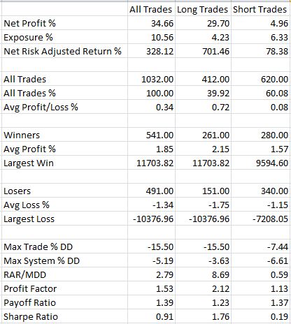
Total trades have increased from 458 to 1032 and net profit has increased from 13.82% to 34.66%. Short trades have increased to 60% of the total and with max system DD (MDD) up to -6.61% on the short side, the RAR/MDD has decreased from 3.80 to 2.79. Profit factor for longs still dwarfs that of shorts (2.12 to 1.13) so I would lean toward trading this long only if multiple signals were allowed.
I will conclude this discussion with a point about position sizing in the next post.
Categories: System Development | Comments (0) | PermalinkTrading System #2–Consecutive Directional Close (Part 2)
Posted by Mark on November 1, 2012 at 07:12 | Last modified: February 4, 2015 10:11In http://www.optionfanatic.com/2012/10/31/consecutive-directional-close-part-1/, I introduced the Consecutive Directional Close trading system. Today I will begin the backtesting in order to see whether this might be worth trading live.
For starters, I will backtest SPY with x = 3 and n = 5. Recall that the two variables are number of consecutive closes (x) either up or down to trigger a short or long trade, respectively, and the number of days to hold the trade (n).
Other backtest settings include:
–Initial account value $1M
–Position size $100K
–$8 commission for each transaction
–Date range 1/29/1993 through 8/30/2012
–Subsequent buy/sell signals ignored once in a trade
Here are the initial results:
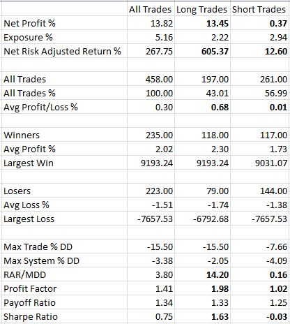
Table 1
With this variable combination, the system does look to be profitable but what really jumps out at me is a huge differential between long and short trades. Profit Factor for shorts is 1.02, which is barely profitable (probably not after slippage). Considering that 57% of all trades were short trades, I would strongly consider trading this long only, cutting exposure by 5.16% to 2.22%, and losing only a fraction of the net profit.
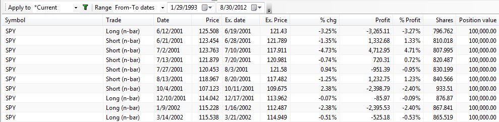
One thing I often wonder about is the final backtest setting to ignore subsequent signals once in a trade. Below are 10 consecutive trades beginning 6/12/2001 with this setting:
Contrast this with 10 consecutive trades beginning 6/12/2001 without this setting:
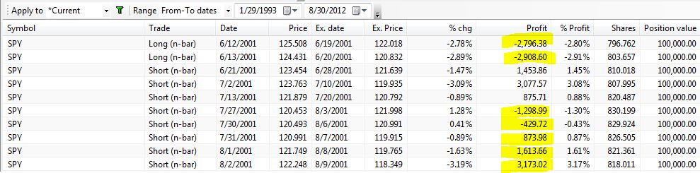
The yellow highlighting indicates subsequent trades that would not have been taken with the setting included. In the first case, an additional trade the following day compounded the initial loss. In the second case, additional trades taken on each of four successive days after the first resulted in a net profit rather than loss.
I will talk more about the implications of this in the next post.
Categories: Backtesting | Comments (3) | PermalinkTrading System #2–Consecutive Directional Close (Part 1)
Posted by Mark on October 31, 2012 at 06:01 | Last modified: October 24, 2012 06:17The next strategy I wish to develop is based on Rule 2 in Larry Connors’ 2009 book Short Term Trading Strategies That Work.
For lack of a better name, I am calling this the “Consecutive Directional Close Trading System.” If you come up with something more catchy then please pass it along.
Connors’ claim is as follows:
> From 1995-2007, after the SPX has dropped three days in a row, it has risen more
> than 4 times its average weekly gain over the next five trading days.
>
> And, after the SPX has risen three days in a row, it has on average lost money over
> the next five trading days.
Two system variables jump out at me immediately. The first variable to test is number of consecutive closes in the same direction (e.g. up or down). The second variable to test is number of days to hold the trade. In thinking back to the SPY VIX trading system, I will test {3, 4, 5, 6, 7} for both variables. This will give me 25 sets of results to study.
SPY is one of many tickers I can imagine using to test this system. I could also test other broad-based US indices like QQQ and IWM. I could also test international ETFs and other asset classes. I could also test SPX-inclusive stocks in order to generate a more complete distribution of trades.
In my next post, I will start testing this system on SPY.
Categories: System Development | Comments (2) | PermalinkDrive the Monte Carlo to Consistent Trading Profits
Posted by Mark on October 29, 2012 at 08:02 | Last modified: October 16, 2012 08:05With backtested trade results in hand for the SPY VIX system, Monte Carlo simulation can help me determine how much capital I can safely trade with the system.
Some approaches to position sizing are based on maximum drawdown (MDD). In Day Trading Futures Online (2000), Larry Williams suggests dividing account balance by margin per contract plus (1.5 x MDD) to determine number of contracts.
Monte Carlo simulation is a technique that can offer more statistical clarity about potential results. Rather than simply assuming the worst future DD to be 50% worse than the backtested MDD, Monte Carlo simulation uses multiple trials and randomization to determine probabilities.
Historically, Monte Carlo simulation was first used by scientists working on the atom bomb. The technique was named for the Monaco resort town renowned for its casinos where games of chance rule the day and has been used in many fields including engineering, insurance, the environment, and finance.
In trading system development, Monte Carlo simulation generates equity curves by randomizing the order of backtested trades thousands of times (or more). The sample distribution of system statistics can then be studied. By using the MDD seen in any randomly shuffled backtest rather than just one specific ordering of historical data, I can quantify my confidence level about future system statistics such as MDD.
Monte Carlo simulation suggests the ordering of outcomes in the past is just one possible history out of an infinite number of equally possible histories. Position sizing based on the average(s) or extreme would serve me best. Out of 10 trades with win loss sequence W-L-W-L-W-W-W-L-W-W, I could have seen W-W-L-L-L-W-W-W-W-W in which case the DD would have been much worse. Monte Carlo analysis will tell me the probability of this taking place.
Categories: System Development | Comments (2) | PermalinkTrading System #1–SPY VIX (Part 10)
Posted by Mark on October 26, 2012 at 09:05 | Last modified: October 15, 2012 10:04In http://www.optionfanatic.com/2012/10/25/trading-system-1-spy-vix-part-9, I presented a MAE graph that damaged any hopes for implementing a protective stop-loss. Today I want to nail this down and make a decision.
The MAE graph can only hint indirectly about an optimal stop-loss level. A graph of the subjective function vs. different stop levels is more definitive. As with other graphs of the subjective function, what I want to see is a high plateau region rather than spikes or trends. Below, RAR/MDD is plotted vs. stop-loss where the latter is varied from 0% to 20% by 0.5% increments:
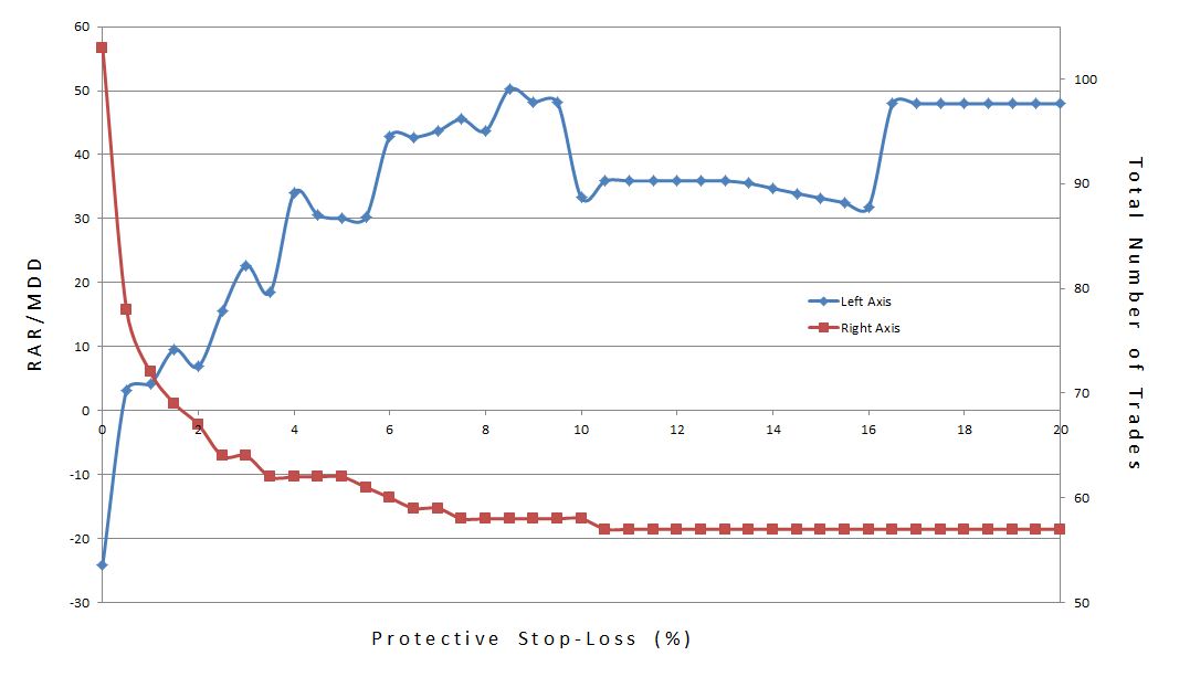
The blue line trending from low to high with a dip in the middle suggests that the system becomes more profitable as the stop-loss is relaxed from zero. The graph clearly shows why tight stops are seldom recommended. While the middle is a plateau region, the fact that it is a valley rather than a peak suggests it is less profitable than a wider stop.
The dip is explained by one trade that had a MAE of 16.45% with a final loss of 0.2%. A stop level up to 16.45% would have caused this trade to exit at the stop level (locking in a loss up to 16.45%). Once the stop level exceeded 16.45%, however, the trade was allowed to rebound and lose the modest 0.2%.
The red line, which indicates total number of trades, decreases as the stop-loss increases. This is because the more often trades are stopped out, the more additional days are freed up for new trades to be opened. Recall that this system only trades one open position at a time.
In conclusion, I do not feel any protective stop-loss should be used with this system at all. I will discuss this more in the context of position sizing.
Categories: Backtesting | Comments (0) | PermalinkTrading System #1–SPY VIX (Part 9)
Posted by Mark on October 25, 2012 at 10:15 | Last modified: October 12, 2012 09:01In http://www.optionfanatic.com/2012/10/20/trading-system-1-spy-vix-part-8, I settled on x = 5 to complete selection of the three parameter values for the SPY VIX trading system. It’s not ready for prime time just yet. Today I will begin exploration into Maximum Adverse Excursion (MAE).
I described the process I am about to undertake in http://www.optionfanatic.com/2012/10/24/maximum-adverse-excursion. Focusing specifically on x = 5, y = 25%, and z = 10, here is a scatter plot of P/L by maximum drawdown (MDD):
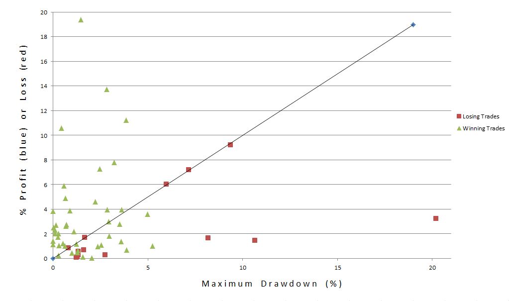
The triangles and squares are results of the 57 trades. The higher the point, the greater the profit (green) or loss (red). The farther to the right, the greater the MAE. The [roughly] 45-degree line is called the loss diagonal, and it represents the maximum loss for red squares. Losing trades can never be above the line because the most they can lose is the most they were ever losing (MDD).
A stop-loss would be represented by a vertical line on the graph. Any losing trades to the right of the vertical line would then move to the intersection of the vertical line and the loss diagonal. Any winning trades to the right of the vertical line would become red squares (losing trades) with height equal to the intersection between vertical line and loss diagonal.
What I want to see in order to implement a stop-loss is more of the former that lie above that intersection than below it and few of the latter. Red squares to the right of the vertical line and above the intersection are trades that would be stopped out for a decreased loss (+1 for system). Red squares to the right of the vertical line and below the intersection represent losing trades that would be stopped out before having a chance to recover (-1 for system). Green triangles to the right of the vertical line represent winning trades that would be stopped out for losses before being able to recover into profit (-1 for system).
I don’t see a good place to draw the vertical line such that the +1’s substantially outweigh the -1’s.
Before dismissing a potential stop-loss for this system altogether, I will undertake one more analysis in the next post.
Categories: Backtesting | Comments (0) | PermalinkMaximum Adverse Excursion
Posted by Mark on October 24, 2012 at 06:53 | Last modified: October 9, 2012 11:13I’ve reached the point with the SPY VIX trading system where I need to analyze maximum adverse excursion (MAE).
MAE is a technique published by John Sweeney in 1997 (John Wiley & Sons, Inc.) that measures the farthest a trade ever goes against you. For long (short) trades, this is calculated with the difference between entry price and the lowest low (highest high) price ever seen during the life of the trade.
MAE is very important from a risk management perspective to help determine potential benefit of a protective stop. A scatter plot of maximum drawdown (MDD) for each backtested trade by final trade profit/loss should be studied. If there is an MDD level beyond which few trades ever end up profitable then it may be useful to keep a protective stop at that level. This may lessen some extreme losers while preserving most of the winners.
The difference between MAE and MDD is that MAE pertains to each individual trade whereas MDD may pertain to an individual trade or a series of trades made by a system.
From a risk management perspective, MAE and MDD both address trader tolerance. Both measure “the farthest X ever goes against you.” Consider the broad stock market as an example. Over the last several decades, the broad market has returned roughly 6% per year. Every now and then, the market crashes and loses 40-60% (or more!) of its value. The MDD is essential to understand because that moment of worst loss is when I will be a nervous wreck, unable to sleep at night, or contemplating a jump out of the nearest 10-story window. If I can’t tolerate the MDD (or MAE) then at best, I won’t be able to reap the benefits of a profitable trade[ing system]. At worst, I may end up suffering catastrophic loss.
In my next post, I will begin to analyze MAE for the SPY VIX trading system.
Categories: System Development | Comments (3) | Permalink