Trading System #1–SPY VIX (Part 8)
Posted by Mark on October 23, 2012 at 01:41 | Last modified: October 9, 2012 06:53In http://www.optionfanatic.com/2012/10/19/trading-system-1-spy-vix-part-7, I finalized values for y (25%) and z (10). Today, I want to make a final decision on x.
From statistical tables in http://www.optionfanatic.com/2012/10/16/trading-system-1-spy-vix-part-5 and http://www.optionfanatic.com/2012/10/19/trading-system-1-spy-vix-part-7, I have cherrypicked just the rows corresponding to y = 25% and z = 10:
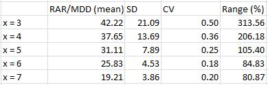
As trade length increases, exposure will increase and RAR will consequently decrease (assuming all else remains equal). This explains the trend lower in RAR/MDD as x increases from three to seven. If I want the most concentrated returns then I should aim for the smallest x-value.
Stability of RAR/MDD across different values of z increases with trade length as evidenced by the trend lower in CV and Range (%) as x increases from three to seven. This suggests I should aim for the largest x-value.
I am favoring x = 5, which will provide a decent RAR/MDD and stability therein.
Since RAR/MDD can obscure Net Profit, I want to add one additional column to the above table:
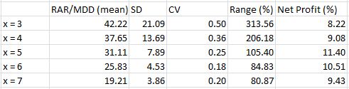
I am somewhat surprised to see Net Profit trail off when x > 5 because the longer the trade, the more opportunity for profit to accumulate. It is possible that after five days mean reversion has occurred and no further edge is available.
The average number of trades for y = 25% is 55.7 (range = 34) across all values of z. This is not a large sample size. If it weren’t for the preponderance of positive numbers across all 150 systems and the trend toward more concentrated profit at higher y-values then I might abort this system altogether and look for something with more backtesting data.
Given all these considerations, I feel comfortable implementing SPY VIX with x = 5, y = 25%, and z = 10.
Categories: Backtesting | Comments (1) | PermalinkHighlights of System Development
Posted by Mark on October 22, 2012 at 06:33 | Last modified: October 8, 2012 09:16Today I want to review a couple major points that have been covered in my last two blog posts.
Trading represents a dream because I am able to work for myself from the comfort of my own home on my own schedule. As hard as it is in this economy to get any job, to get a gig like this will demand out of me something the vast majority of others are not putting forth. This just makes sense because otherwise, everyone would be doing it! For starters, I must be willing to put in extensive legwork at every turn whether or not it ends up being required.
Trading as a business can never coexist with laziness.
The trading landscape for independents is like a hot desert littered with mirage. I am constantly bombarded with alluring returns and trading strategies that sound good. Greed pushes me to gamble with speculative trades on a whim. Wishful thinking accelerates the process. Other cognitive heuristics also combine to stack the deck against me.
System development must be extremely thorough to flush out any oversights that may lead to false profit expectations. One could say the whole point of system development is to highlight the arbitrary and determine it to be lucky or good: discard the former and implement the latter.
This was the idea behind realizing the need to backtest 3-, 4-, 6-, and 7-day trades before moving forward with a 5-day SPY VIX trading system. Failure to perform these additional steps could leave me unknowingly chasing an illusion. When lucky, traders will eventually find out by losing precious capital and often going bust. When good, traders are able to stay in the game.
All trading recommendations, whether technical strategies or stock screens, are due only one response: backtesting within the confines of a complete system development process to assess how likely they are to perform in the future. This is a labor-intensive process where many false leads and dead ends potentially await.
Categories: System Development | Comments (0) | PermalinkTrading System #1–SPY VIX (Part 7)
Posted by Mark on October 19, 2012 at 08:09 | Last modified: October 7, 2012 11:27In http://www.optionfanatic.com/2012/10/17/trading-system-1-spy-vix-part-6, I determined that for x = 5, y = 25% produced the best backtesting results for z-values between 6-15 (see first paragraph of http://www.optionfanatic.com/2012/10/18/laziness-dissected for a refresher on the SPY VIX trading system). I now want to see if this holds for x = 3 to 7.
Here is the graph and statistical analysis (lowest stability numbers in bold) for x = 3:
Here is the graph and statistical analysis (lowest stability numbers in bold) for x = 4:
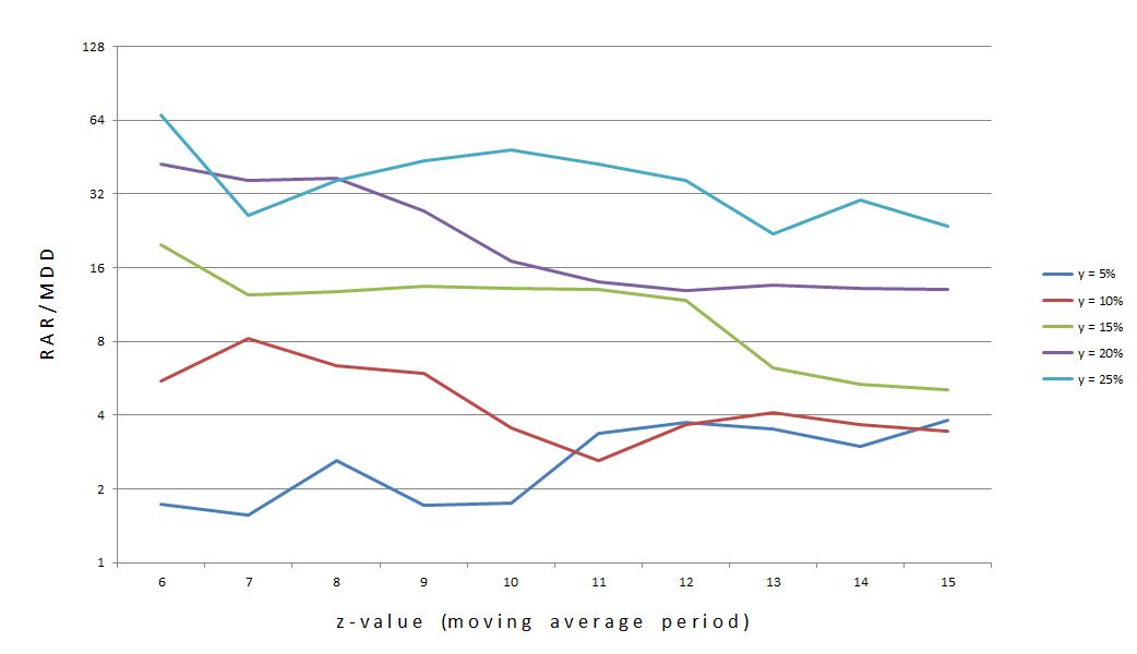
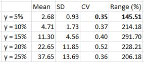
Here is the graph and statistical analysis (lowest stability numbers in bold) for x = 6:
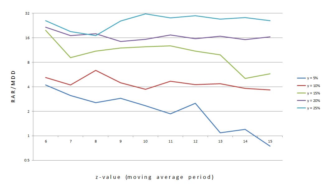
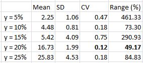
Here is the graph and statistical analysis (lowest stability numbers in bold) for x = 7:
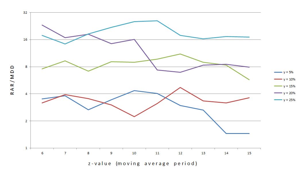
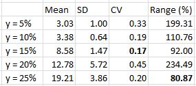
Which value of y had the most stable curves as measured by lowest CV (SD / mean) and lowest Range (%) statistics?
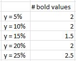
No edge there…
The y = 25% curve prints the largest RAR/MDD for most values of z on all graphs. Out of 50 total backtested systems, RAR/MDD was largest along the y = 25% curve 44 times (by random chance alone, one would expect 10). Six times, y = 20% resulted in a larger RAR/MDD value. These six cases occurred with z = 6 (once), z = 7 (three times), or z = 8 (twice). Never did this occur for z-values of 9-15.
In conclusion, y = 25% is as consistent as any other y-value across all values of x and z. Furthermore, y = 25% reliably scores highest on the subjective function RAR/MAD. In looking at the five y = 25% curves, I would choose z = 10 as the center of the most consistent plateau region where the curve is least likely to fall off “precipitously” at neighboring z-values. Even if the y = 25% curve does fall off, however, RAR/MAD is still very likely to be larger than curves of any other y-value and in all cases would still have generated respectable profit.
Categories: Backtesting | Comments (2) | PermalinkLaziness Dissected
Posted by Mark on October 18, 2012 at 11:50 | Last modified: January 14, 2019 10:38Back in Part 1, I described the SPY VIX trading system as having three variables. The system trades when VIX is y% extended from its z-SMA with an x-bar stop.
Full disclosure: I don’t want to consider the x-bar stop as a system variable. So the trade lasts five days. That seems routine and unlike a technical indicator I employ where I set the critical value to be tested. Why bother checking x for validity? Besides, I have already entertained y-values from 5 to 25 (five total) and z-values from 6 to 15 (10 total). Allowing x to vary from three to seven, for example, would increase the number of potential systems from 50 to 300. Furthermore, keeping one variable constant would now leave two to vary. This suggests employment of college Calculus rather than high school Algebra in order to study performance.
It doesn’t take much introspection to discover that this bellyaching is simply a matter of laziness. At some level, most people tend toward laziness. This may be the primary reason why most new traders fail in the first 1-5 years. They think this is an undiscovered country where hard work doesn’t exist. They are eager and willing to pay hundreds to thousands of dollars on trading books, investment webinars, or educational programs that promise consistent profits in 10 minutes per night or a couple hours per month. They are fertile ground for scammers and con artists, alike.
I have written this before and I’ll write it again: no free lunch is available in the world of trading and investment. I’m up against institutions with billions of dollars at their disposal and highly-educated quant teams with thousands of advanced degrees between them all focused exclusively on gaining the slightest bit of Edge. The easy way out is no longer a viable option. Screw the ego-laden label of “busywork…” when it comes to labor-intensive, painstaking tasks, I need to shut my eyes, puff out my chest, and rush headlong into the pile so I can get the job done.
The x-bar stop: in focus with my next post.
Categories: System Development | Comments (2) | PermalinkTrading System #1–SPY VIX (Part 6)
Posted by Mark on October 17, 2012 at 05:50 | Last modified: October 6, 2012 07:18In http://www.optionfanatic.com/2012/10/16/trading-system-1-spy-vix-part-5/, I took a close look at the subjective function RAR/MDD by % extended across moving average length (z). I will continue that analysis today.
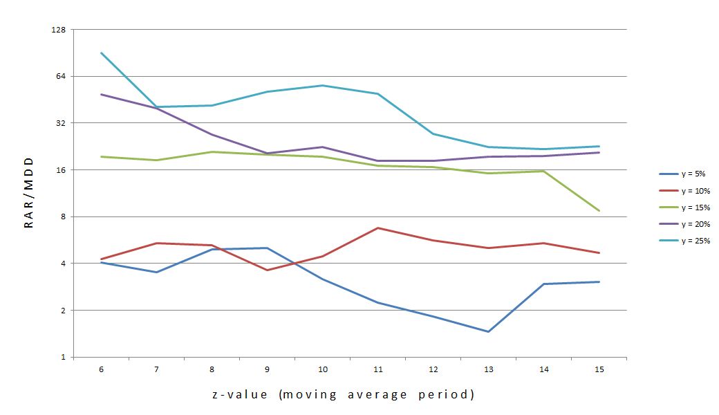
Let me begin by reposting Figure 1 from my last post:
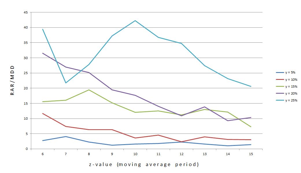
The statistics showed that y = 25% (top curve) is actually the flattest of the five. Perhaps this graph is more convincing:
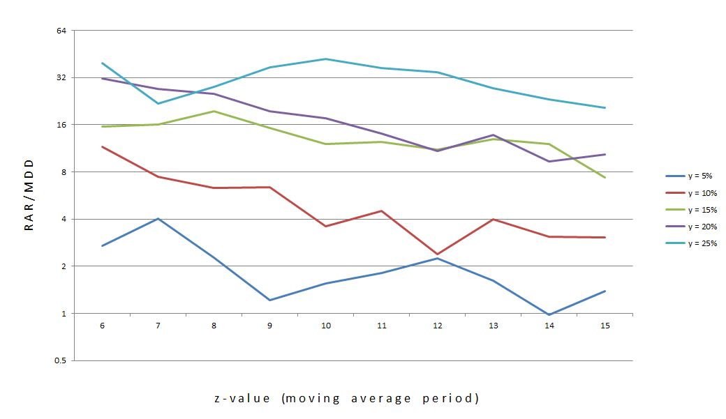
Do you see the difference? The y-axis is logarithmic in the bottom one, which means any given length represents the same multiplier rather than addend. Each tick on the y-axis multiplies the previous y-value by two rather than adding five. This eliminates distortion caused by widely-ranging (in percentage terms) values.
In addition to choosing y = 25%, I will choose z = 10. This is roughly the center of the middle, high plateau region of the curve.
Going back to Table 1 in http://www.optionfanatic.com/2012/10/16/trading-system-1-spy-vix-part-5/, another observation about these 25% extended systems is the low number of trades. Indeed, a regression analysis shows that total number of trades and % extended are highly correlated (R-squared = 0.8921). On average, these 25% extended systems traded 55 times over 20 years, which is just over 2.5 trades/year.
Despite trading infrequently, these 25% extended systems have been very profitable in the past. Profit factor (PF) is positively correlated with % extended with an R-squared value of 0.7516. The 25% extended systems have the highest average PF of all with an average of 3.13.
To recap, I have 2.5 trades/year x 5 days/trade = 11 days/year and 11 days/year x 1 year / 252 trading days = 4.4%. If I can find 10 more systems that have a good basis for diversification then I can have be invested on roughly 50% of all trade-days (# trades x trading days invested) with good probability for concentrated profits (high PF). A good basis for diversification includes mean-reverting and trend-following systems along with different (non-correlated) asset classes.
I’m not done developing this system, though. In the next post, I will discuss the x-bar stop.
Categories: Backtesting | Comments (1) | PermalinkTrading System #1–SPY VIX (Part 5)
Posted by Mark on October 16, 2012 at 06:40 | Last modified: October 5, 2012 07:07The subjective function is now in hand: RAR/MDD. I will now recreate the results presented in http://www.optionfanatic.com/2012/10/02/trading-system-1-spy-vix-part-3-2 and redo the consequent analysis.
Here are the results for the top 30 parameter combinations as sorted by RAR/MDD:
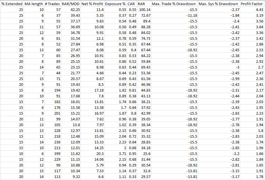
Table 1
My first observation is that a cluster of 25% extended systems sit right at the top. Indeed, running a linear regression analysis on all 50 systems shows that % extended and RAR/MDD are correlated with an R-squared value of 0.77 (R-squared > 0.80 is typically considered “strongly correlated”).
This makes logical sense as a mean-reversion trading system. Mean-reversion systems are based on the idea that the farther the rubber band gets stretched, the more likely it is to snap back [to the mean]. The more extended VIX gets above or below the VIX moving average, the more likely SPX is to move higher or lower, respectively. This was also seen [less clearly] in the graph of Net Profit % (http://www.optionfanatic.com/2012/10/03/trading-system-1-spy-vix-part-4/).
If I break down systems by z-value (moving average period), then the results look like this:
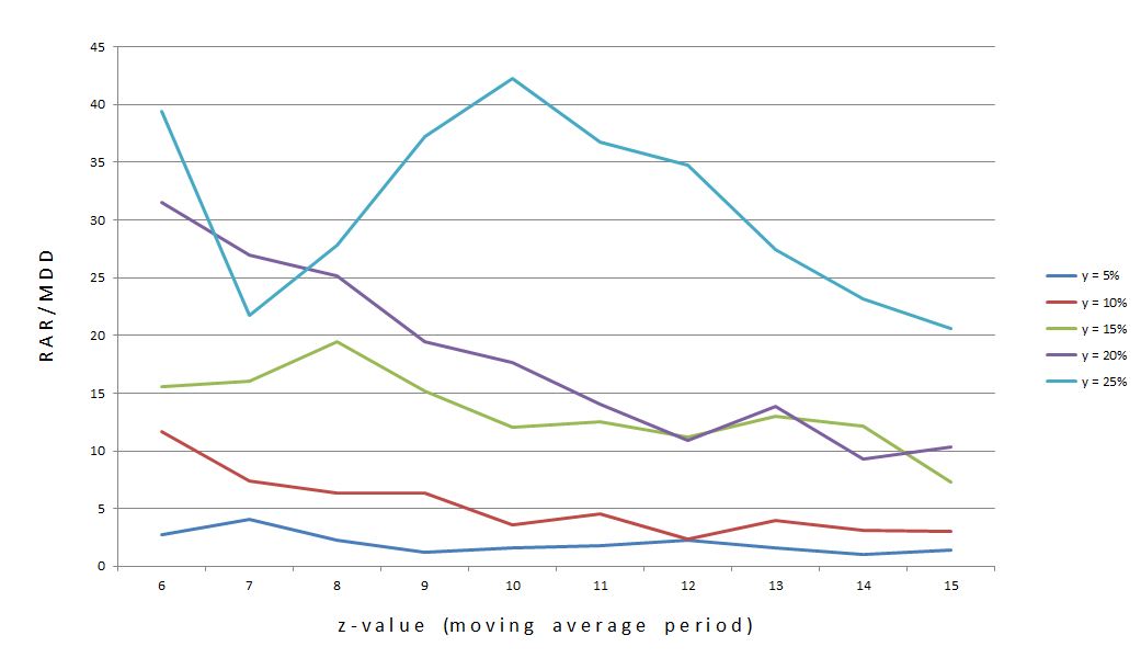
Figure 1
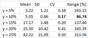
Keeping in mind that I want to see plateau regions rather than spike regions, the bottom curve (y = 5%) looks best. The statistics do not bear this out, however:
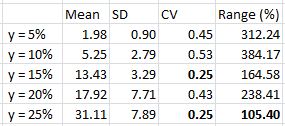
Table 2
Mean = average RAR/MDD
SD = Standard Deviation
CV = Coefficient of Variance (SD / mean)
The lower the SD, the flatter the curve. Even more important is to interpret SD as a percentage of the mean since the means vary over 15-fold. By that metric, y = 25% is the most consistent.
Indeed, y = 25% has a greater RAR/MDD over the entire range of z values. Even the lowest RAR/MDD for y = 25% (at z = 7) is greater than the highest RAR/MDD for y = 15% (at z = 8). Given these observations, y = 25% seems to be the best choice.
I will continue this analysis in the next post.
Categories: Backtesting | Comments (0) | PermalinkMotion to Dismiss System Development?
Posted by Mark on October 15, 2012 at 06:07 | Last modified: October 4, 2012 06:38I now have the subjective function from http://www.optionfanatic.com/2012/10/12/the-subjective-function-part-6/. Before I move on and apply this to the SPY VIX trading system, I want to briefly discuss one other point that threatens to derail system development.
In my last post (see above), I mentioned the following with regard to high-profit, infrequently-trading (i.e. “surgical”) systems:
> Ideally, I would like to take advantage of the time one such system is not in the market
> by trading with another surgical system that is in the market. I am therefore in the
> market more frequently with systems that deliver concentrated profits.
When trading with surgical systems, the only way to achieve a reasonable percent return on the entire portfolio in a risk-controlled manner is to combine them.
Statistically speaking, this is the employment of non-correlated systems (i.e. low R-squared values). With two non-correlated systems, one system may be making money while the other is flat (i.e. out of the market) or one system may be losing money while the other is making a bit more. The catch is that R-squared is calculated based on historical data. During explosive market conditions, one system may make money when the other system suddenly loses much more. Even worse, both systems may become correlated and lose money together.
While these are threatening possibilities, without more details I can’t say it’s reason to dismiss system development altogether. You could look at a long historical backtesting period to determine how often these conditions occur. When they occur may be generalizable to a particular type of market condition. You could explore the possibility of including a failsafe filter–for example, suspending trade of a mean-reverting system in case of powerful breakout or breakdown. Whether the markets traded by these systems are the same or different could also affect the severity of this threat.
I will continue analysis of the SPY VIX trading system in my next post.
Categories: System Development | Comments (0) | PermalinkThe Subjective Function (Part 6)
Posted by Mark on October 12, 2012 at 04:51 | Last modified: October 1, 2012 06:31I unmasked the systems in yesterday’s post (http://www.optionfanatic.com/2012/10/11/the-subjective-function-part-5). Prior to that I made all my observations about the graphs shown in http://www.optionfanatic.com/2012/10/09/the-subjective-function-part-3. Once and for all, the time has arrived to select the subjective function.
On one hand, I like a system that trades more and presents more opportunity for profit. This sort of system has a profit factor (PF) just over 1.00 and grinds out a small profit in each of many trades. This would be insert #3.
On the other hand, I prefer systems that are surgical in their efficacy. These generate infrequent trades and have larger PFs (e.g. over 1.50 or 2.00). Ideally, I would like to take advantage of the time one such system is not in the market by trading with another surgical system that is in the market. I am therefore in the market more frequently with multiple systems that each deliver concentrated profits. I prefer this model.
The risk of using surgical systems to make the equivalent dollar profit as a frequent trading system is that larger position sizing must be employed. Although the likelihood is that these trades will end up profitable, in case the next trade results in MDD the larger position size could result in catastrophic loss.
I want a subjective function that takes into account both profit and DD. A system may have had minimal DDs in backtesting but as one author on system development described, your worst DD is always ahead of you. If the subjective function does not factor in DD then I fear the Risk of Ruin.
Therefore, I will choose RAR/MDD (insert #1) as the subjective function. By using RAR instead of compound annualized return, I also like the fact that the more a system is out of the market, the more it is rewarded.
Categories: System Development | Comments (1) | PermalinkThe Subjective Function (Part 5)
Posted by Mark on October 11, 2012 at 09:05 | Last modified: January 18, 2013 07:59Yesterday in http://www.optionfanatic.com/2012/10/10/the-subjective-function-part-4, I began the analysis of graphs posted in http://www.optionfanatic.com/2012/10/09/the-subjective-function-part-3 to determine the subjective function. Today I will make my remaining observations.
Equity curve #3 posts the greatest profit of all three curves. This profit of 20.3% is roughly 283% greater than equity curve #2 and about 78% greater than equity curve #3. This relates to my previous observation of also being in drawdown (DD) more than the other two. If curve #3 is in DD more than the others but is drawing down from a much greater net profit then I may still be happier with this system than with the others.
With regard to maximum DD (MDD), insert #2 has the edge. MDD here is -1.8%, which is 25% less than insert #1 (-2.4%) and 18% less than insert #3 (-2.2%). Lower DD means less risk. I could increase position size a bit to make for comparable MDDs and a larger profit for insert #2. While this suggests I could increase position size slightly, though, it certainly would not make up the 283% greater profit equity curve #3 has over #2.
Do not forget that in order to secure the 283% profit, insert #3 has over 10 times as many trades as insert #2 and is therefore in the market over 10 times longer. Theoretically, this is greater risk that could turn sour on us in the future even though it did not significantly do so in 19.5+ years of backtesting.
Time to unmask the systems:
–Insert #1 (y = 25, z = 10) generated the highest profit factor of all 50 systems.
–Insert #1 generated the highest risk adjusted return (RAR).
–Insert #1 generated the highest RAR:MDD ratio.
–Insert #2 (y = 25, z = 6) is the system that generated the lowest MDD.
–Insert #3 (y = 10, z = 6) is the system that generated the highest net profit.
So which is better?
Categories: System Development | Comments (1) | PermalinkThe Subjective Function (Part 4)
Posted by Mark on October 10, 2012 at 07:31 | Last modified: October 1, 2012 06:03I’m in the process of trying to determine the subjective function, as defined in http://www.optionfanatic.com/2012/10/05/the-subjective-function-part-1. In http://www.optionfanatic.com/2012/10/09/the-subjective-function-part-3, I showed three inserts to help us in this determination. I will analyze those today.
Let me start by emphasizing the need to study relative differences in net profit, drawdown, and other details between the three inserts. If I focus on absolutes then I will be disappointed. The one and only goal of this study is to determine which I prefer most.
In looking at the equity curves, my first observation is that they are all upward sloping to the right. I should hope so. Each insert corresponds to the system that performed best on a different metric. Whichever curve I like the best corresponds to the metric I will use to evaluate systems. This will be the subjective function. Since each of these systems is the best in some respect, I am glad to see they are all profitable.
Equity curves #1 and #2 have many discernible plateau (horizontal) regions as opposed to #3, which seems to have more incremental changes. This corresponds to the total number of trades. Inserts #1, #2, and #3 have 57, 37, and 399 total trades, respectively. On this metric alone, I prefer a system that trades more because that means more opportunity for profit.
Drawdown curves #1 and #2 have a much smaller blue area than #3. This means #3 spends more time in drawdown and less time at new equity highs. I really like new equity highs because they make me feel like a successful trader. The broad market does not make all-time highs very often.
Equity curve #1 is lower now than it was around the beginning of 2009. This seems like a negative. However, each of these systems goes into drawdown periodically and curve #1 did hit a new high roughly 1+ centimeters ago (on my screen), which is only a couple fractions of a centimeter more than the other two. Curve #1 just happens to be in greater drawdown (-0.59%) than the other two but by no means it this drawdown remarkable. This observation may be disregarded.
I will continue this analysis in my next post.
Categories: System Development | Comments (2) | Permalink