The Subjective Function (Part 3)
Posted by Mark on October 9, 2012 at 05:37 | Last modified: September 28, 2012 07:30I keep coming up with quirky analogies for different aspects of the system development process. In http://www.optionfanatic.com/2012/09/19/trading-system-1-initial-assessment-part-1/ on 9/19/12, I talked about a Motion to Dismiss. On 10/8/12 (http://www.optionfanatic.com/2012/10/08/the-subjective-function-part-2), I talked about visiting the eye doctor. As promised, today I will present some graphs for study to help determine the subjective function.
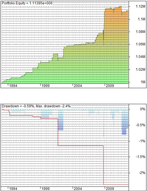
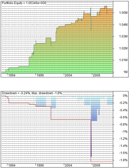
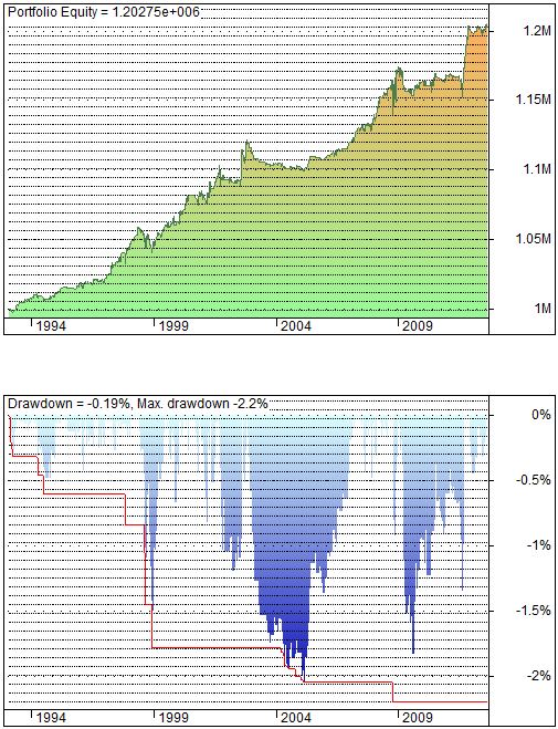
The following inserts show two graphs each. On the top is the equity curve itself: a plot of account value over time beginning with $1M and traded with a $100K position size. On the bottom is the drawdown (DD) curve. DD is zero whenever the account is at a new high. The red line on this graph tracks the max DD ever seen over the whole time period. You will see the red line dip to levels not seen in the blue graph but that is only because the DD was too short to be seen in the blue graph. If you were able to zoom in and magnify then you would see the blue graph dip to those levels.
As you look the following three inserts, imagine that you are studying the performance of your investment account over time. Which would you feel best about? Note details such as relative net profit (final value is shown in the upper left of the top curves), relative severity of drawdowns (current drawdown at the right edge of the bottom curves is shown in the upper left of the bottom curves), relative time between new equity highs, number of horizontal periods (indicating no current trade), etc.
Now without further ado, let me present…
Insert #1:
Insert #2:
Insert #3:
I will analyze these graphs based on my preferences in the next post.
Categories: System Development | Comments (1) | PermalinkThe Subjective Function (Part 2)
Posted by Mark on October 5, 2012 at 17:25 | Last modified: October 4, 2012 06:35My last post (http://www.optionfanatic.com/2012/10/05/the-subjective-function-part-1) defined the subjective function. Today I want to present another perspective on the subjective function by explaining what I previously missed.
The gist of my previous posts is that all traders are looking for the same general thing. “Consistent profitability over time” is a phrase I have written many times over. Yes, Trader A may be looking for the supercharged exponential returns that carry the risk of heavy drawdowns while Trader B is more conservative and will sacrifice returns to minimize drawdown. Aren’t they both basically looking for consistent profitability over time, though?
No.
I now see that Trader A and Trader B are looking for decisively different things. My “consistent profitability over time” is what Trader B seeks. Trader A, however, is in effect buying a lottery ticket and hoping for the big payout. If financially savvy then Trader A is playing this with a limited percentage of the total portfolio so as not to go completely bankrupt. Trader B might be all-in with proper asset allocation.
My previous lack of understanding might reflect an inadequacy of language itself. I suspect we just don’t have enough terms to reflect the variety of individual preference for investment returns. Compound annual growth rate (CAGR), drawdown (DD), and flat times translate directly to features seen on equity curves but others do not (e.g. profit factor, Sharpe and Sortino ratios). Equity curves reflecting the same CAGR or DD can look wildly dissimilar, however. The pictures tell more than words can describe.
Moving beyond language in this manner is what Dr. Bandy recommends in Quantitative Trading Systems (2007) to determine the subjective function. After running the trading system optimization, scroll through the different equity curves to find the ones you like best. Note which metrics score highest on your favorite equity curves and voila! You have the subjective function. This is not unlike a visit to the eye doctor where you endure an exhausive series of “which lens is better: one or two? 1 or 2? 2, or 1? 2, 1?”
In fact, let’s do that: a visit to the optometrist’s office, and more, when we return.
Categories: System Development | Comments (1) | PermalinkThe Subjective Function (Part 1)
Posted by Mark on October 4, 2012 at 19:03 | Last modified: October 4, 2012 06:34I’ve mentioned multiple times that in trading system development we’re looking for consistent profitability over time. To do this, identification of the “subjective function” is a prerequisite.
Much of the direction to my current work is owed to Dr. Howard Bandy. You can read about him here: http://www.linkedin.com/pub/howard-bandy/b/b44/270 . In his book Quantitative Trading Systems (2007), Bandy defines the “objective function” as:
> A single-valued measurement of the fitness of a trading system. Optimization
> techniques are guided by maximizing the value of the objective function.
He also writes:
> Only you can decide which trading systems are good and which are not.
> Selection of the objective function is a management decision and must
> be made prior to extensive model development. The objective function
> itself is not a candidate for optimization.
What does this mean?

System trading is the epitome of Yin and Yang! Beginning on 5/7/12 (http://www.optionfanatic.com/2012/05/07/strategies-vs-systems-part-i/), I wrote a number of blog posts discussing discretionary vs. systematic trading. The upshot was that discretionary trading is subjective and systematic trading is objective. This may be true but at the heart of a somewhat objective system development process is the very personal selection of Bandy’s objective function. For this reason, I have chosen to call it the subjective function.
All this subjective function talk may seem highly theoretical but it really boils down to something quite simple. On 10/4/12 (http://www.optionfanatic.com/2012/10/04/trading-system-1-spy-vix-part-4/), study the y-axis to see my subjective function: net profit (%). I proceeded to discuss the best combination of parameters by performance on that measure.
The only problem is that I failed to go through the process of determining my subjective function before implementing it.
Stay tuned for further discussion and a possible detour in upcoming posts.
Categories: System Development | Comments (3) | PermalinkTrading System #1–SPY VIX (Part 4)
Posted by Mark on October 3, 2012 at 23:03 | Last modified: October 4, 2012 06:32Today I will begin to analyze results of the SPY VIX trading system optimization study. Please refer to Tables 2A and 2B from http://www.optionfanatic.com/2012/10/02/trading-system-1-spy-vix-part-3-2 for the backtest results.
My first observation is that each of the 50 parameter combinations leads to a profitable system! Net profit % ranges from 4.66% to 20.30%. Remember that the issue we’re ultimately trying to address is how probable it is that the system we are backtesting will generate profit going forward. All parameter combinations backtesting profitably makes me more confident that the chosen system will be profitable in live trading than if all parameter combinations did not backtest profitably.
While this conclusion may seem obvious, it does head off the tendency to infer more from the observation than is actually presented. Beginning (and seasoned!) traders are all-too-often eager to enter the market with any half-decent excuse for a [potentially] winning system, open their bags, and let the money fall in. This is the allure/mirage of Wall Street (otherwise known in human nature terms as “greed”). The harsh reality is quite to the contrary. It takes great effort to develop profitable systems and we have just begun. Perhaps “all backtested systems profitable” is one of our checkpoints but our checklist better be much longer if we are to have a realistic chance of being good and not lucky (or worse).
Following the course of evolutionary operation, I now want to analyze returns of each y-value individually:
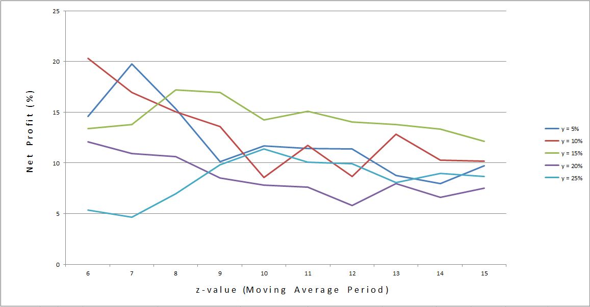
What line(s) has large plateau regions rather than spike regions? The red line seems to dive early (e.g. from z = 6-10) and then flatten out. The blue line goes up and then way down before flattening. The green line seems relatively flat. The light blue line rises early on and then retraces half that rise. The purple line falls gradually but seems pretty flat from z = 9-15.
This eyeball method is consistent with a cursory statistical analysis:
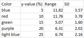
Green and purple lines vary the least (flatness).
The one problem I have with this method is the percentage nature of the dependent variable. That is, falling from 20(%) to 15(%) or 10(%) to 5(%) are both a range of 5% but the former is a 25% difference whereas the latter is a 50% difference.
That criticism aside, based on these data I would choose y = 15% and z = 10 (near the middle of plateau regions).
I will continue this analysis in future posts.
Categories: Backtesting | Comments (1) | PermalinkTrading System #1–SPY VIX (Part 3)
Posted by Mark on October 2, 2012 at 08:01 | Last modified: September 21, 2012 09:21In http://www.optionfanatic.com/2012/10/01/trading-system-1-spy-vix-part-2/ (10/1/12), I continued the discussion of evolutionary operation by reviewing optimization. Today I will begin the optimization process for the trading system.
For the initial backtest, I am going to leave x fixed at 5 days and, as mentioned in the last blog post, vary y from 5-25 in increments of five [e.g. 5 (percent), 10, 15, 20, or 25] along with z from 6-15 in increments of one. Other backtesting assumptions were discussed in “Trading System #1–Backtesting Assumptions” from 9/14/12. The only change here is that I will take long and short SPY trades when VIX is “overbought” and “oversold,” respectively.
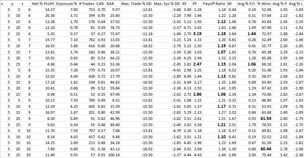
Table 2A
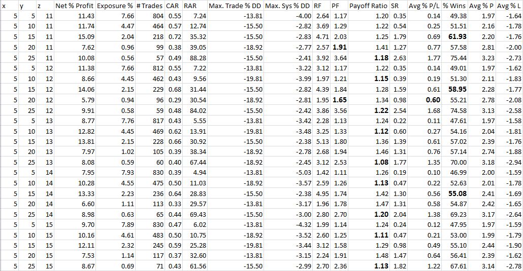
Table 2B
I abbreviated headings to make the Table font larger:
CAR = Compound Annualized Return (%)
RAR = Risk Adjusted Return (%) = CAR / Exposure %
Max. Trade % DD = Largest intratrade drawdown (%) (denominator is position size)
Max. Sys % DD = Largest portfolio drawdown (%) (denominator is current account value)
RF = Recovery Factor = Net profit / Max. System DD (higher is better)
PF = Profit Factor
Payoff Ratio = Average win / Average loss (second term of PF calculation)
SR = Sharpe Ratio
Avg % P / L = Average % gain or loss per trade
Avg % P = Average % profit on winning trades
Avg % L = Average % loss on losing trades
Several trends are evident from studying these results. The numbers in bold and larger font are unexpected values with regard to these trends. Feel free to take some time to peruse the Tables.
In my next post, I will begin the data dissection.
Categories: Backtesting | Comments (2) | Permalink
Trading System #1–SPY VIX (Part 2)
Posted by Mark on October 1, 2012 at 06:04 | Last modified: September 21, 2012 06:58In http://www.optionfanatic.com/2012/09/28/trading-system-1-spy-vix-part-1/ (9/28/12), I introduced the concept of evolutionary operation and began to talk about the different variables present in this trading system. Today I want to continue that discussion from the perspective of optimization.
Investopedia.com defines optimization as:
“…the process of adjusting one’s trading system in an attempt to make it more effective. These adjustments include changing the number of periods used in moving averages, changing the number of indicators used, or simply taking away what doesn’t work.”
In the system development process, optimization is going to allow me to look at performance metrics for every combination of specified parameter values. In the present context, I will allow x to vary from 3-7 in increments of one [e.g. 3 (days), 4, 5, 6, or 7]. I will allow y to vary from 5-25 in increments of five [e.g. 5 (percent), 10, 15, 20, or 25]. I will allow z to vary from 6-15 in increments of one. The result of this process will be summary statistics for 5 * 5 * 10 = 250 trading systems.
The goal of optimization is not to find out which set of parameter values performed the best in order to trade those going forward. This is called “curve-fitting” and the reason optimization has gotten a bad name in some circles. The more variables you have and the greater the number of total parameter value combinations, the more unlikely you are to see similar performance in the future as seen in the most profitable backtest.
Rather, the goal of optimization should be to assess the performance landscape from one combination of parameter values to the next. Going back again to http://www.optionfanatic.com/2012/09/28/trading-system-1-spy-vix-part-1/ (9/28/12), I want to know if these performance graphs have spike regions or plateau regions. If they have spikes then I will discard them, considering performance to be lucky rather than good. If they have plateau regions then I want to choose parameter values near the middle of those plateaus (margin of safety).
In my next post I’ll start running the numbers.
Categories: System Development | Comments (2) | PermalinkTrading System #1–SPY VIX (Part 1)
Posted by Mark on September 28, 2012 at 05:31 | Last modified: October 1, 2012 05:35With the “motion to dismiss” now denied, the next step is to lay the groundwork for developing this strategy into a trading system.
As a review, the trading strategy is based on two claims. First, five days after the CBOE Volatility Index (VIX) closes 5% or more below its 10-day simple moving average (SMA), the S&P 500 index (SPX) has lost money on average. Second, when the VIX closes 5% or more above its 10-SMA, SPX has outperformed the average week better than 2-1 over the next five trading days.
The current system in development offers three variables to be backtested: x-bar stop y% extended from its z-SMA. In this case, we have used x=5 (five-day trades), y=5, and z=10 (VIX closing 5% above/below its 10-SMA). What we want to see in backtesting is solid results with these values. We also want to see solid results when we slightly change these values, though.
The process of “evolutionary operation” looks to keep one variable constant while changing another to see its effect on system performance. Graphically speaking, we want to plot some measure of performance (e.g. net profit) vs. the one variable being changed:
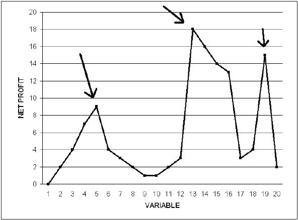
This does not have the appearance of a robust system because slight changes in the variable drastically affect net profit. Whether a moving average is four periods vs. five or 14 periods vs. 15 should not matter. If one value appears magically improved in the midst of mediocre results then those backtested profits are likely a matter of luck rather than the system taking advantage of consistent opportunity (and subsequent future profits).
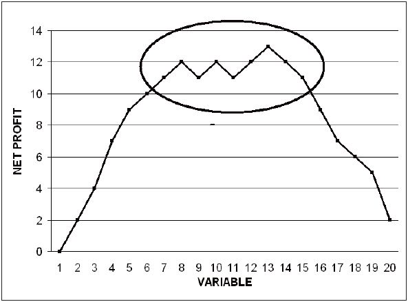
This is what we hope to see. All values from 6-15 produced solid profit for this trading system. Rather than the spikes in the previous graph we see a plateau region in this one. This should be a necessary (but not sufficient) condition for a system we might trade in the future with real capital.
These graphs were adapted from Tomasini and Jaekle (2009).
In my next post I will continue this discussion in terms of optimization.
Categories: System Development | Comments (2) | Permalink
Trading System #1–Initial Assessment (Part 6)
Posted by Mark on September 27, 2012 at 06:38 | Last modified: September 21, 2012 06:55In my post http://www.optionfanatic.com/2012/09/25/trading-system-1-initial-assessment-part-5/ (9/25/12), I finished up my analysis of the overbought VIX trading strategy. Today I want to study the claim of avoiding SPY when VIX is oversold, which I described in http://www.optionfanatic.com/2012/09/13/trading-system-1-introduction/ (9/13/12).
Do 5-day long trades in SPY actually lose money if placed when VIX is over 5% or more below its 10-SMA (“oversold”)? I have included these results in the third column in order to compare with all 5-day SPY trades and 5-day SPY trades only when VIX is “overbought”:
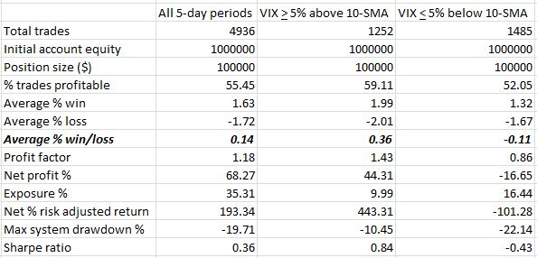
Indeed, the oversold VIX strategy loses money. Average % win is much smaller (1.32%) and the lower % trades profitable (52.05%) contributes to a negative profit factor and negative Sharpe ratio.
Now having substantiated both of the initial claims, I feel more confident about putting forth time and effort to try and develop a trading system. I will continue with these steps in my next post.
Categories: Backtesting | Comments (0) | PermalinkTrading System #1–Initial Assessment (Part 5)
Posted by Mark on September 25, 2012 at 07:09 | Last modified: September 21, 2012 06:54We have been studying the difference between 5-day long trades in SPY with daily entry vs. with entry only when VIX closes at least 5% above its 10-SMA (“overbought”). Going back to Table 1 from my post http://www.optionfanatic.com/2012/09/19/trading-system-1-initial-assessment-part-1/ (9/19/12), today we will discuss the remaining results.
The overbought VIX strategy gets a slight edge with regard to % profitable: 59.11% to 55.45%. In a broad sense, systems are usually trend-following or mean-reverting (i.e. sell when the market is strong and buy when the market is weak). Trend-following systems typically have a lower % of profitable trades whereas mean-reverting systems have a higher % of profitable trades. Trend-following systems typically have a much better average % win (for winning trades) to average % loss (for losing trades) ratio, however. This is the tradeoff. Recall that % profitable trades and average gain/loss are the two components of profit factor (PF) calculation.
The final statistic is the one I highlighted with bold: average % win/loss. In looking at Table 1, this statistic seemed to be the coup de grace for the “overbought” VIX strategy. With both strategies having similar winning percentages, the “overbought” VIX strategy dominated with a 0.36% vs. 0.14% average % win/loss. This difference is also reflected in the PF although the difference is not as clear (1.43/1.18 << 2). The difference is reflected in the SR but as previously discussed SR is shroud in more complexity and controversy as a meaningful number. One needs to have studied many systems before developing an intuitive understanding of how SR differences may reflect system performance.
In my post http://www.optionfanatic.com/2012/09/13/trading-system-1-introduction/ (9/13/12), I mentioned the internet claim that “when VIX closes 5% or more above its 10-SMA, SPX has outperformed the average week better than 2-1 over the next five trading days.” Based especially on this average % win/loss statistic, I consider that claim to be verified.
This now leaves us to determine SPX (SPY) performance when VIX is “oversold.” I will address this in the next post.
Categories: Backtesting | Comments (2) | PermalinkTrading System #1–Initial Assessment (Part 4)
Posted by Mark on September 24, 2012 at 06:20 | Last modified: September 19, 2012 06:12Today I will continue to compare the SPY daily long strategy with vs. without an overbought VIX filter by discussing Sharpe Ratio (SR).
The Sharpe Ratio (SR) is one of the most commonly referenced measures of risk/return. It is calculated as the difference between the average return and the risk-free rate divided by the standard deviation of all returns.
The numerator of the SR describes “excess return.” The better the average return of the system the greater this number will be. The sign of SR will be determined by the numerator and any potentially profitable system must have a positive SR.
The denominator rewards systems that have higher consistency of returns. Typically when a system performs well, positive returns are consistent (e.g. closing at set profit targets). When the market goes awry for a system, feel lucky if you get taken out at your stop-loss point. In many cases with violent market moves, a gap may jump far beyond a stop-loss point before the trade closes. For this reason, more poorly performing systems have a larger variability of returns and therefore larger denominator.
A primer on how to calculate SR with Microsoft Excel is seen here: http://investexcel.net/214/calculating-the-sharpe-ratio-with-excel/ .
The SR has been highly criticized in financial circles and should therefore be taken with a grain of salt. For one thing, rewarding consistency of returns (e.g. 2% per month rather than 12% one month and 0% the other 11 months) means short option premium strategies often get high SRs. Short option strategies have catastrophic risk, however, that many other trading strategies do not (think Long Term Capital Management in 1998). What is also debatable is that the SR penalizes variability of returns whether that variability is profit or loss. A strategy that returned 2% in 11 months and 12% in one month would reflect similarly in the denominator as one that returned 2% in 11 months and -8% in one month.
In the current study, buying SPY when VIX is “overbought” results in a much better SR of 0.84 vs. 0.36. As is often the case with other system statistics, SR is often negatively correlated with exposure. This means in order to get the desired net profit out of your portfolio, a single highly profitable system won’t be enough. The goal should be to find multiple systems with large PFs or large SRs to work together.
Categories: Backtesting | Comments (0) | Permalink