Crude Oil Strategy Mining Study (Part 4)

Last time, I presented results for the first factor: R(ules). Today I continue presenting results from my latest strategy mining study on crude oil.

The second factor, Q(uality), has a significant main effect on performance (see hypothesis[2]). Not only are best strategies an improvement over worst, the best strategies are [marginally] profitable. Top strategies (n = 816) average PNL +$87, PNLDD 0.34, Avg Trade $1.38, and PF 1.05. As mentioned in the third-to-last paragraph here, none of these numbers approach what might be regarded as viable for any OOS results. They sure would be damning if they landed on the side of loss, though.

D(irection), the third factor, has a significant effect on performance: Avg Trade -$17 (-$57) and PF 1.01 (0.94) for short (long) trades. This should not be surprising since CL fell from $84.60 to $54.89 during the incubation period creating a downside bias (hypothesis[3]). What should be surprising is that as with PNLDD and Avg Trade in Part 3 (second table), Avg Trade is negative for both long and short trades while PF < 1 only for the latter.

A glance at the variable distributions helps me to better understand this apparent sign inconsistency. Avg Trade has an approximately Normal distribution with sub-breakeven (negative) mean. PF has a skewed distribution with a right tail out to 2.37 and left tail down to 0.22. In other words, the right tail goes 1.37 units above breakeven (1.0) while the left tail only goes 0.78 units below breakeven (1.0). This should produce some upward pressure on average PF to exceed 1.0.

The fourth factor, P(eriod), does not have a significant effect on performance. I find it peculiar that the 2007-2011 training period generates significantly more trades than 2011-2015, but I’m not sure why and I don’t think it really matters.

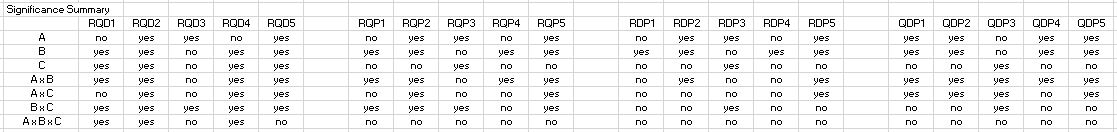
A significant 2-way interaction effect is seen between R and Q. Performance improves slightly in looking from two to four rules across the worst strategies whereas performance declines much more when comparing two to four rules across the best strategies. This interaction is the first graph shown here.

A significant 2-way interaction effect is seen between Q and D. Performance improvement is much greater for top vs. bottom strategies on the long side whereas performance improvement is marginal for top vs. bottom strategies on the short side (like the second graph in the link provided just above).

A 3-way interaction effect is seen between R, Q, and D. This is significant for Net PNL, PNLDD, and Avg Trade and marginally significant (p = 0.057) for PF. I’m not going to try and explain this interaction nor am I going to undertake a 4-way ANOVA by hand to screen for a 4-way interaction that I probably wouldn’t understand either.

I will continue the discussion next time.

Crude Oil Strategy Mining Study (Part 3)

Today I will start to analyze results of my latest study on crude oil.

I ended up running four 3-way ANOVA tests. Recall the factors I am testing:

• R(ules: two or four)
• Q(uality: best or worst)
• D(irection: long or short)
• P(eriod OOS: 2007-2011 or 2011-2015)

I am running these analyses on five dependent variables:

• Net PNL
• PNL / max DD
• Avg Trade
• Profit Factor (PF)
• Number of trades

The first four are performance-related while the last is for curiosity.

Along the lines of “conventional wisdom,” here are some hypotheses:

1. Four-rule strategies should outperform two.
2. Best strategies should outperform worst.
3. Long (short) strategies should outperform if the market climbs (falls) during the incubation period.
4. Order of IS and OOS periods should not make a difference since strategies are selected on performance over both.
5. Number of trades should be fewer for 4-rule than for 2-rule strategies (fifth-to-last paragraph here).
6. The software is capable of building profitable strategies.

Here are the results:

Let’s begin with somewhat of an eye-opener: 2-rule strategies averaged PNLDD 0.15 and PF 0.99 vs. 4-rule strategies with PNLDD –0.02 and PF 0.95. I think this is surprising for two reasons. First, the simpler strategies did better (see hypothesis [1]). Second, the signs are misaligned for the 2-rule group. I checked for sign agreement on every strategy; how can overall PNLDD reflect profit when overall PF reflects loss? The answer is because strategy drawdowns along with the relative magnitude of gains/losses all differ. When averaged together, sign agreement may no longer follow.

Consider this example of two strategies with two trades each:

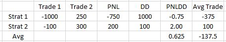
Signs align between PNLDD and Avg Trade for each strategy, but when averaged together the signs do not align. PNLDD may be a decent measure of risk-adjusted return, but it cannot be studied alone: sign must be compared with Avg Trade (or PNL). Forgetting this is like adding numerators of fractions with unequal denominators (i.e. wrong).

If I do nothing else today, then this discovery alone makes it an insightful one.

Getting back to the first factor, R does not significantly affect PNL or Avg Trade. PNL is almost identical over 816 strategies (-$4,014 vs. -$4,015). This is a good argument for risk-adjusted return (like PNLDD) as a more useful metric than straight PNL even given constant contracts (one, in this study). With regard to Avg Trade, 2-rule strategies outperform $33 vs. -$41. This difference is not significant.

Here’s something else to monitor: all results so far are negative (see hypothesis [6]).

I will continue next time.

Main Effects vs. Interaction Effects in Statistics

I am almost ready to analyze the effects of different independent variables on strategy performance. Before I proceed, I think main versus interaction effects are important enough to illustrate.

One example is shown below:

Drug treatment appears to have no main effect on pain relief score. If I graph the data showing both genders, though:

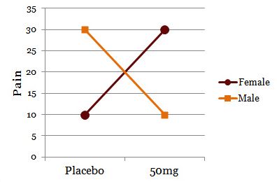
I now clearly see the effect of drug on pain relief depends on gender. This is a significant interaction despite no main effect.

Consider this example:

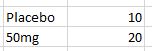
The drug appears to have a main effect because 50mg results in more pain relief than placebo. To simply collapse the data across gender and claim a main effect, though, shows only part of the story:

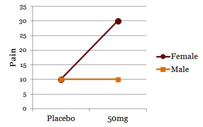
The effect of drug on pain relief clearly depends on gender. For men or women, the drug has no effect or helps, respectively.

While these are 2-way interaction effects, higher-order interaction effects can occur between three or four variables. A 3-way interaction is a 2-way interaction that varies across levels of a third variable. A 4-way interaction is a 3-way interaction that varies across levels of a fourth variable. These get harder to conceptualize as the number of factors increases.

Interaction effects limit generalizability of main effects. I can easily comprehend “A causes B.” An interaction effect means I must qualify: “A causes B, but only when C is… [high or low].”

From a statistical standpoint, my crude oil study does not make for an easy analysis. I am interested in the four factors of strategy quality (best vs. worst), number of rules (two vs four), training period (OOS beginning vs end), and trade direction (long vs. short). With regard to interaction effects, I have seen written in multiple places that 4-way and even higher-order interactions are very difficult to interpret and are rarely meaningful.

Rather than attempting a 4-way analysis of variance (ANOVA: a statistical test), I could run four 3-way ANOVAs or six 2-way ANOVAs. This would simplify interpretation of interaction effects. What doesn’t change, however, is the fact that I am still looking at the effects of four different factors. A 3-way or 4-way interaction is still possible regardless of whether my statistical test has the capability of measuring it. I wonder if I am just blocking out part of my visual field in order to better understand what I do see, which may not be the most legitimate course of action.

I will continue next time.

Why is Curve Fitting Such a Bad Word?

I have been trying to get more organized this year by converting incomplete drafts into finished blog posts. Some of these are from out in left field, but I am publishing them anyway on the off chance someone might be able to benefit.

In the second paragraph here, I said “optimization” is sometimes a bad word. It is specifically a bad word when used to mean curve fitting, which relates back to this draft I wrote in July 2019.

—————————

Is it curve-fitting or curve fitting? Whatever it is, it’s a bad word when used in these parts.

The process of curve fitting, though, is not a bad process but rather a branch of mathematics.

Wikipedia gives us:

     > Curve fitting[1][2] is the process of constructing a curve, or
     > mathematical function, that has the best fit to a series of data
     > points,[3] possibly subject to constraints.[4][5] Curve fitting
     > can involve either interpolation,[6][7] where an exact fit to
     > the data is required, or smoothing,[8][9] in which a “smooth”
     > function is constructed that approximately fits the data. A
     > related topic is regression analysis,[10][11] which focuses
     > more on questions of statistical inference such as how much
     > uncertainty is present in a curve that is fit to data observed
     > with random errors. Fitted curves can be used as an aid for
     > data visualization,[12][13] to infer values of a function where
     > no data are available,[14] and to summarize the relationships
     > among two or more variables.[15] Extrapolation refers to the
     > use of a fitted curve beyond the range of the observed data,
     > [16] and is subject to a degree of uncertainty[17] since it
     > may reflect the method used to construct the curve as much
     > as it reflects the observed data.

When used without validity, curve fitting turns bad. Looking to the past for viable strategies with the hope of applying them in the future makes sense. However, the past is unlikely to match the future and I have no idea of knowing how similar the two may be. The more I try to curve fit a strategy to the past, the less likely it is to work in the future.

The true goal of trading system development is to provide enough confidence to stick with a strategy through times of drawdown in order to realize future profit (see end of third paragraph here). However, if the strategy is poorly suited for the future because it is curve fit to the past then I will definitely lose money trading it. Curve fitting is a bad word in this respect.

Crude Oil Strategy Mining Study (Part 2)

Last time, I detailed specific actions taken with the software. Today I will start with some software suggestions before continuing to discuss my latest study on crude oil.

This backtesting took over 30 hours. For studies like this, implementing some of the following might be huge time savers:

• Allow execution (e.g. Monte Carlo analysis, Randomized OOS) on multiple strategies from the Results window at once.
• Offer the option to close all Results windows together* since each Results exit requires separate confirmation.
• [Alternatively] Allow multiple [strategy] selections to be retested on a particular time interval and create one new Results window with all associated data. This would save having to re-enter a new time interval [at least two entries for year, in my case, and sometimes 3-4 entries when a month and/or date got inexplicably changed. This occurred 4-8 times per page of 34 strategies during my testing] for each and every retest in addition to saving time by closing just one Results window per page (rather than per strategy).
• Include an option in Settings to have “Required” boxes automatically checked or perhaps even better, add a separate “Re-run strategy on different time interval” function altogether. Retesting a specific 4-rule strategy involves checking “Required” for each rule, but testing the same strategy on different time intervals encompasses “Required.”
• Offer the option to close all open windows (or same-type windows like “close all Monte Carlo Analysis windows?” “Close all Randomized OOS windows?”) when at least n (customizable?) windows are already open. Exiting out of non-Results windows can take noticeable time when enough (80-90 in my case) need to be consecutively closed.

My general approach to this study is very similar to that described in Part 6:

• Train over 2011-2015 or 2007-2011 with random entry signals and simple exit criteria.
• Test OOS from 2007-2011 or 2011-2015, respectively (two full sets of strategies).
• Identify 34 best and 34 worst performers over the whole 8-year period for each set.
• Retest over 2015-2019 (incubation).
• Re-randomize signals and run simulation two more times.
• Apply the above process to 2-rule and 4-rule strategies.
• Apply the above process to long and short positions.
• Include slippage of $30/trade and commission of $3.50/trade.

In total, I recorded incubation data for 2 * 34 * 2 * 3 * 2 * 2 = 1,632 strategies in this study: 816 each were long/short, 2-rule/4-rule, best/worst strategies, and OOS beginning/end (each category is itself mutually exclusive, but categories are not mutually exclusive of each other). I enter data with relative speed and accuracy, but mistakes can definitely be made. As another study improvement over the last, I therefore ran some quality control checks:

• Compare NetPNL and PNLDD for sign alignment (e.g. both should be positive, negative, or zero).
• Compare NetPNL and Avg Trade for sign alignment.
• Compare NetPNL and PF for alignment (if NetPNL < 0 then PF < 1; if NetPNL > 0 then PF > 1).
• Compare PNLDD and Avg Trade for sign alignment.
• Compare PNLDD and PF for alignment.
• Compare Avg Trade and PF for alignment.
• Verify that Avg Trade ~ (NetPNL / # trades).
• Screen PF for gross typos (e.g. 348 instead of .48; extremes for all occurrences ended up being 0.22 and 2.37).

I will continue next time.

* — This may be difficult because I want only the re-run Results windows—not the
       whole simulation Results window closed. Perhaps this could be offered in Settings.
       I have written elsewhere (paragraphs 4-5 here) about the potential utility of
       retesting strategies on separate time intervals; this might be a widely appreciated
       feature by algo traders.

Crude Oil Strategy Mining Study (Part 1)

Today I continue a blog mini-series focused on putting context around trading system development. I am trying to better understand what can be expected from strategies that look good in the developmental phases.

With each subsequent study, I am discovering nuances and better learning the software. My previous study is described here. In the current study, I have attempted to compile pieces from previous studies and avoid earlier mistakes.

As I learn, the exact methodology varies from study to study. I previously studied equities while I now move forward with crude oil. The following study is my first to include a dedicated stop-loss. What follows is also my first study featuring a highest high (lowest low) stop for long (short) trades. Subsequent studies may not include these. Regardless of the differences, my ultimate goal is to walk away with some big-picture conclusions based on recurring themes found inside the numbers.

Full details on the following study is included in Mining 8, but I will go into extensive detail here.

My process with the software was very repetitive:

• Enter correct settings (e.g. long/short, HHV/LLV stop, 2/4 rules, OOS at beginning/end), clear and select Random 1000 entry signals, and remove signals in Time category.
• Run continuous simulation x 5′.
• Sort by All: PNLDD and screenshot worst [34*] strategies.
• Eye results to make sure no duplicate strategies included (discard and replace).
• Transcribe 34* strategy numbers into spreadsheet.
• Sort by All: PNLDD and screenshot best [34*] strategies.
• Eye results to make sure no duplicate strategies included (discard and replace).
• Transcribe 34* strategy numbers into spreadsheet.
• Select “Re-run strategies with adjustments,” adjust backtest dates, and [4-rule strategies only] require all rules.
• Maximize Results window, right click x2,* and select “All.”
• Group together first six* Results windows then every four thereafter with first on top, second below top row of overall Results window (seen in background), and subsequent windows somewhere below.
• Once all 34 re-runs complete, select Results windows four (six for first group) at a time and sequentially drag on screen with Net PNL vertically aligned.
• With four (or six) tiled on screen,* drag Excel spreadsheet directly below fourth Results window and transcribe Net PNL, PNLDD, # trades, Avg Trade, and PF.
• With six tiled, transcribe stats for first four, drag spreadsheet just above Results windows 5-6, transcribe stats for these, and close out 5-6.
• [Drag spreadsheet below fourth Results window if six originally tiled and] Close out Results windows 1-4.
• Run Randomized OOS, noting in spreadsheet strategies that pass two consecutive runs (second paragraph here).
• Run Monte Carlo (MC) analysis, noting in spreadsheet strategies with resample average DD less than backtested DD (seventh paragraph here).
• Close all MC and Randomized OOS windows.
• Sort by All: PNLDD worst to best.
• Repeat Randomized OOS and MC analysis steps for worst strategies then close all associated windows.
• Repeat steps for re-running strategies over incubation and transcribe OOS2 (third bullet point) performance stats.
• Re-randomize entry signals, remove time-related signals, and enter or check to make sure correct settings still entered.
• Rinse and repeat.

I will continue next time.

* — Many of these steps are reflective of my particular screen size, resolution, etc.

Stepping Back to Walking Forward (Part 1)

Reflecting on recent studies, I’m starting to see a bridge between data mining and walk-forward (WF) optimization.

Let me begin by discussing the assumption that all trading systems break. I will not be able to verify this myself until I have developed a respectable sample size of viable strategies [I have zero thus far] with further data on strategy lifetimes. Nevertheless, many gurus talk about continuous system monitoring in case of breakage. Many traders mention it, too.

One explanation for the poor performance I have seen in recent studies (see third-to-last paragraph here) could be that the incubation period is too long. I’ve been testing good-looking strategies over a subsequent four-year period. What if the average lifetime of a profitable strategy is six months? Averaging over four years when real outperformance may be limited to six months could result in overall mediocrity.

Recall my discussion in this second- and third-to-last paragraph where I suggested the most important feature of strategy performance might be a maximal number of profitable runs over the complete backtesting period. This echoes WF with the exception of reoptimizing parameter values: here I want to stick with one constant strategy all the way through.

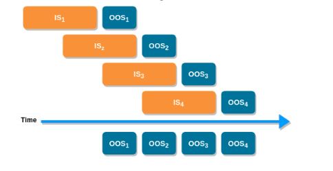
A shorter average strategy lifetime means validation or incubation should be tested over shorter time intervals. The WF process seems perfectly suited for this: test over relatively brief OOS periods, slide the IS + OS window forward by those brief increments, and concatenate OOS performance from each run to get a longer OOS equity curve. I like the following image to illustrate the concept:

I started to describe the data-mining approach to trading system development with regard to how it diverges from the WF process here. I feel I may now have come full circle albeit with the one slight modification.

As I struggle to rationalize the Part 7 results (first link from above), I can shorten the incubation period or leave it unchanged in subsequent studies.

Perhaps I am suggesting a new fitness function altogether: percentage of OOS runs profitable.

Backtracking a bit, I think much of this evolved because I have yet to see validation data for the different stress tests. Such data is not forthcoming from the product developer who says in a training video, “at the end of the day, we are still competitors and I have to keep some things to myself.” This is data I will have to generate on my own.

Mining for Trading Strategies (Part 7)

Although my next study aimed to correct the mistake I made with the previous [long] study, I accidentally mined for short strategies. This was illuminating—as described in these final three paragraphs—but did not address the comparison I really wanted to make (see Part 6, sixth paragraph).

Given the fortuitous discovery I made from that short study, though, I proceeded to repeat the long study by switching around IS and OOS periods. I trained strategies on 2007-2011 and incubated from 2015-2019. I tested only 4-rule strategies expecting to find worse performance due to an inability to effectively filter on regime [which may have taken place in the previous study]:

Results are mixed. Beginning outperforms on Net PNL and Avg. Trade. End outperforms on PNLDD and PF. None of these differences are statistically significant.

This does not seem to be consistent with my theory about mutually exclusive regimes. That would be one regime controlling 2007-2011, a different regime controlling 2011-2015, and just one ruling 2015-2019.

In the face of a persistent long bias, such regimes would not exist: long strategies would be profitable whereas short strategies would not. As a general statement, this is true. Looking more closely, however, it certainly is not. 2007-2009 included a huge bear (benefiting shorts) while 2009 to (pick any subsequent year) benefits long strategies.

And if it’s tough to figure out equity regimes, then good luck finding anything of a related sort when it comes to CL or GC where words like “trend” and “mean reversion” don’t even begin to matter (based on my testing thus far).

Where to go from here?

• I should repeat the last study with 2-rule strategies to make sure I don’t get any significant differences there either.
• I could require a regime filter for the 4-rule strategies just in case none/few have been implemented.
• I need to better understand the short strategies. It’s one thing to find strategies that pass IS and OOS. It seems to be quite another to find strategies that do well on a subsequent OOS2. Performing well in OOS2 is what ultimately matters.

I have one other troubling observation to mention. Although the long strategies in all three studies (including that from Part 5) incubated profitably on average, performance does not begin to approach what we might require from OOS in any viable trading strategy. I did see flashes of brilliance among the 4-rule strategies (6, 9, and 10 strategies for each of three long studies posted PNLDD over 2.0 with a few excursions to 6 and one over 14!). On average, though, 203 top long strategies over eight years averaged a PF ~1.21 and PNLDD ~0.8 over four years to follow of a consensus bull market.

And don’t forget that we don’t have context around the 1.21/0.8 without comparable numbers for long entries matched for trade duration (Part 6, sixth paragraph).

Forget all the pretty pictures (see second paragraph here); if this is an accurate representation of algorithmic trading then those who say you’re not going to get rich trading equities certainly weren’t kidding!

Stability

Continuing on with my year-long organization project, this is an unfinished draft from January 2019 on stability.

—————————

The extent to which stability seems to be left out of trading system development is alarming.

I worry that lack of [a] stability [derivative] has the potential to disrupt the entire backtesting endeavor. “Past performance is no guarantee of future returns” may be a microcosm of everything I am to say below.

Trading system development often looks at a large sample size of trades and gives averages. One problem with looking at the average across a large time interval is that the local averages at different points within the whole interval may vary greatly. Suppose I find the average ATR is 15. That doesn’t tell me whether 80% of occurrences are at 15 or whether 2% of occurrences are at 15 with 49% each at 5 and 25. Huge difference!

If I use a VIX filter and say “bad things happened with VIX over 30” but this only happened 60 of 4000+ times and most were in 2008 (third paragraph here), then have I added a robust guideline or simply one that is curve fit to the past (i.e. based on something that is unlikely to repeat)? I think one benefit of walk-forward is that by training over the recent past, I won’t get locked into using values that may be historic extremes and cherry-picked over a long period of time. For example, the long-term average for VIX may be 16-18 but in 2017 we went the whole year without seeing 12 and for at least a couple years we only rarely got over that LT average.

Therefore, anytime I’m going to look at historic data and determine a critical value, I need to look at frequency of that value and the distribution of those instances. If I could eliminate the losses of Feb 2018 then it might make for meaningful portfolio performance. However, if Feb 2018 were the only time such an event occurred, then I’m entering into a behavior pattern whereby I insure myself against any unique past event ever seen. This is like mummifying a corpse by placing paper mache over every single square inch of flesh (see third paragraph here) to eliminate exposure. In the end, this is either the Holy Grail (reward without risk) or a flat position (no risk, no reward). I can’t expect to have everything covered.

Rolling averages are a means to assess stability. If I have 16 years of data then an average over the entire 16 years may not be very meaningful. Taking 3-year rolling averages, though, and then looking at what percentage of the 14 rolling periods generate a return in excess of X%, for example, is a better way to describe the whole. The distribution is also important: by percentage return and by date. I don’t want to see anything to suggest the system is broken (e.g. all winners in the first eight years and all losers in the last eight).

Stability also matters with regard to correlation. Correlation is used as support for particular strategies (e.g. intermarket) or creating multi-strategy portfolios. Correlations change, though. I think it would be useful to plot rolling correlations to better understand whether it makes any sense to report static correlations or whether they fluctuate enough to be meaningless.

Mining for Trading Strategies (Part 6)

Last time, I presented some study results with a caveat that the study was flawed. I proceeded to repeat the study.

I used the same methodology:

• Trained over 2011-2015 with random entry signals and simple exit criteria
• Tested OOS from 2007-2011
• Identified ~32 best performers over the whole 8-year period
• Collected performance data over incubation period from 2015-2019
• Re-randomized signals and ran simulation again for total sample size ~64
• Included slippage of $25/trade
• Included commission of $3.50/trade

Here are the results:

The five performance criteria shown are all better for 4-rule than 2-rule strategies. None of the differences are statistically significant (see final paragraph here), however. Perhaps they would become significant with a larger sample size.

The average trade is profitable regardless of group. This is encouraging! I couldn’t help but wonder, however, whether this was due to finding effective strategies or just plain luck. If I had collected data on average length of trade, then it would be interesting to compare this with average long trade of comparable length starting every trading day. The null hypothesis says there shouldn’t be any difference.

For my next study, I intended to reverse the IS and OOS periods to see if the positive performance was the result of aligning regimes for IS and incubation periods. Remember that I developed strategies (i.e. “trained”) over 2011-2015 and incubated over 2015-2019. Most of those eight years were bull market regardless of definition. Would I get similar results if I trained over 2007-2011, which includes a significant bear market cycle, and incubated over 2015-2019 (mostly bullish)?

Unfortunately, I was sloppy in doing this study and tested short positions rather than long. Here are the results:

Like the previous [long] study, all performance criteria favor 4-rule strategies. The Net PNL difference is statistically significant even after applying the Holm method for multiple comparisons. No other metric is significantly different (alpha = 0.05).

As expected, number of trades is significantly different because with more trade rules, the less likely all entry criteria are to be met on any given day.

Did you catch the big difference between this table and the table above?

Performance metrics for the short study are negative and significantly worse (by orders of p-magnitude) vs. the long study.

This is not encouraging and honestly makes me scratch my head a bit. I have this wonderful software that builds well-incubating long strategies but poor-incubating short strategies. Perhaps credit for the long study should not go to the software, but rather to some unknown, serendipitous similarity between the IS and incubation periods. Allowing up to four rules, wouldn’t inclusion of at least one be effective to keep the strategy out of markets during unfavorable environments?

I will continue next time.