My Journey (2019 Update)
Posted by Mark on September 24, 2019 at 09:52 | Last modified: March 27, 2020 11:07My focus has definitely shifted since I took a break from blogging.
2018 was first the losing year since I started trading full-time 11 years ago. That was certainly a wake-up call. I decided my trading approach was too risky to be doing with more than a limited portion of the account (akin to what I discussed in the second paragraph here). As a result, I have traded a small position size all year. While I have been profitable, I have significantly underperformed the benchmark.
My focus has gradually turned toward incorporating other asset classes in addition to equity options. I hope such diversification can increase total returns more than drawdown thereby improving my risk-adjusted return.
One way to accomplish this is to trade a basket of long uncorrelated futures. In other posts, I will detail my reasoning and plan for this strategy. Said discussion also begs for some space devoted to the concept and implications of correlation.
Another way to trade multiple asset classes is to develop multiple trading strategies. I will delve into this next time.
Categories: About Me | Comments (0) | PermalinkBeen a Long Time!
Posted by Mark on September 19, 2019 at 14:53 | Last modified: March 23, 2020 15:13Welcome back!
I’m actually saying that to myself because from your perspective, nothing may be different. Truth be told, however, I took a relatively long (for me, anyway) hiatus from blogging.
Worry not, though: this has happened before!
It happened here.
It happened here.
It happened here.
It’s now happened again.
But as I say with the omnipresent COVID-19, which now dominates the headlines and the structure of our everyday lives, we will get through this. I will ease back into my writing, which should help me go faster. I will relearn WordPress (and perhaps even update). I will relearn what HTML I need to manage the behind-the-scenes formatting of these posts.
And hopefully, I will bring you much more in the way of useful content. I certainly have been doing some interesting stuff, and I would love to be able to bring some of that to you.
Stay safe out there!
Categories: About Me | Comments (0) | PermalinkTesting the Noise (Part 4)
Posted by Mark on September 13, 2019 at 06:16 | Last modified: June 10, 2020 11:36I am now ready (see here and here) to present detailed results of the Noise Test validation analysis.
The strategy counts by market are as follows:
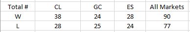
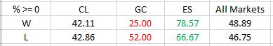
DV #1 (original equity curve positioning within the simulated distribution) breaks down as follows:
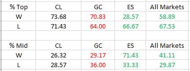
Frequencies are virtually identical for CL regardless of group (winning or losing strategies). Differences are seen for GC and ES with green and red indicating a difference as predicted or contrary to prediction, respectively. The more simulated curves that print above the original backtest, the more encouraged I should be that the strategy is not overfit to noise (see third graph here for illustration of the opposite extreme).
The difference in winning and losing strategies for ES is statistically significant per this website:
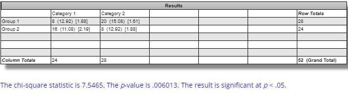
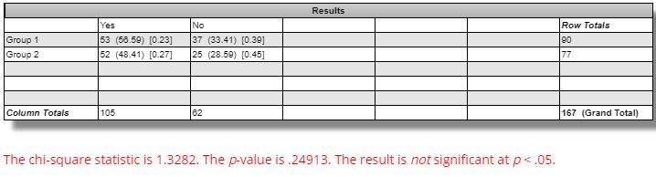
The difference between winning and losing strategies across all markets is not statistically significant:
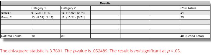
DV #2 (percentages of strategies with all equity curves finishing breakeven or better) breaks down as follows:
The difference seen between winning versus losing GC strategies is marginally significant (questionable relevance and even less so, in my opinion, due to smaller sample size):
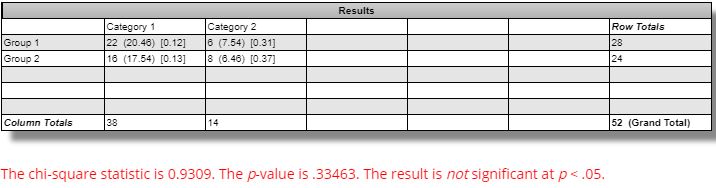
The difference seen between winning versus losing ES strategies is not statistically significant:
DV #3 (average Net Profit range as a percentage of original equity) breaks down as follows:
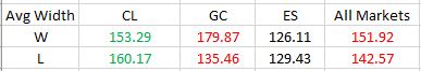
We should expect the simulated equity curves to be less susceptible to noise and therefore lower in range for the winning versus losing strategies. Across all markets, this difference is not statistically significant [(one-tailed) p ~ 0.15]. The difference for GC is statistically significant [t(49) = 2.92, (one-tailed) p ~ 0.003]: in the opposite direction from that expected.
Based on all these results, I do not believe the Noise Test is validated. The reason to stress potential strategies is because of a positive correlation with future profitability. I built 167 random strategies that backtested best of the best and worst of the worst. Unfortunately, I found little difference across my three validation metrics between extreme winners and extreme losers. My ideal hope would have been 12 significant differences in the expected directions. I may have settled for a few less. I got two with only one in the predicted direction.
Perhaps I could at least use Noise Test DV #1 on ES. I might feel comfortable with that if it were not for DV #3 on GC—equally significant, opposite direction—and an overall tally that suggests little more than randomness.
One limitation with this analysis is a potential confounding variable in the number of occurrences of open, high, low, and close (OHLC) in the [two] trading rules. My gut tells me that I should expect number of OHLC occurrences to be proportional to DV #3. A strategy without OHLC in the trading rules should present as a single line (DV #3 = 0%) on the Noise Test because nothing would change as OHLCs are varied. I am uncertain as to how X different OHLCs across the two rules should compare to just one OHLC appearing X times in terms of Noise Test dispersion.
I cannot eliminate this potential confound. However, this would not affect DV #1 and would perhaps only affect DV #2 to a small extent. More importantly, the strategies were built from random signals, which gives me little reason to suspect any significant difference between groups with regard to OHLC occurrences.
Categories: System Development | Comments (0) | PermalinkTesting the Noise (Part 3)
Posted by Mark on September 10, 2019 at 06:10 | Last modified: June 10, 2020 07:05Today I want to go through the Noise Test validation study, which I described in Part 2.
As I was reviewing screenshots for data evaluation, a few things came to light.
The consistency criterion (second-to-last paragraph of Part 2) is not an issue. All 167 strategies were “consistent” according to the Noise Test. When I decided to monitor this, I now wonder if I was remembering back to the Monte Carlo test instead.
Instead of consistency, I realized on some occasions all of the simulated curves were above zero. This percentage became dependent variable (DV) #2 and implies profitability regardless of noise. DV #1 describes where [Top, Mid(dle), or Bot(tom)] the original backtest terminal value falls within the equity curve distribution. DV #3 is net income range as a percentage of terminal net income for the original backtest.
I never saw the original backtest fall in the bottom third of the equity curve distributions (Bot, DV #1). This would be a most encouraging result that the software developers never presented as an example (see Part 1). Thanks for not deceiving us!
I found myself making some repetitive comments as I scored the data. On 19 occasions, I noted the original equity curve to be at the border of the upper and middle third of the distribution. Since equity values were estimated (platform does not have crosshairs or a data window), I simply alternated scoring Top and Mid whenever this occurred. I did not wish to feign more accuracy than the methods provide.
Also taking place on 19 occasions was a single simulated equity curve (out of 101) finishing below zero. One makes a big difference since the criterion is binary: all curves either avoid negative territory or they do not. This occurred 10 times for CL (split evenly between winning/losing groups), four times for GC (split evenly between winning/losing groups), and five times for ES (four winning and one losing strategy).
I recorded one CL strategy with an extremely profitable outlier and one GC and ES strategy, each, with an extremely unprofitable outlier.
I will present and discuss detailed results next time.
Categories: System Development | Comments (0) | PermalinkTesting the Noise (Part 2)
Posted by Mark on September 5, 2019 at 07:21 | Last modified: June 14, 2020 14:01Many unprofitable trading ideas sound great in theory. I want to feel confident the Noise Test isn’t one of them.
One big problem I see with the system development platform discussed last time is a lack of norms. In psychology:
> A test norm is a set of scalar data describing the performance
> of a large number of people on that test. Test norms can be
> represented by means and standard deviations.
The lack of a large sample size was part of my challenge discussed in Part 1. The software developers were kind enough to offer a few basic examples. The samples are singular and context is incomplete around each. I need to validate the Noise Test in order to know whether it should be part of my system development process. Without doing this, I run the risk of falling for something that sounds good in theory but completely fails to deliver.
I will begin by using the software to build trading strategies. I will study long/short equities, energies, and metals. I will look for the top and bottom 5-10 in out-of-sample (OOS) performance for each with OOS data selected as beginning and end (doubling sample size and re-randomizing trade signals to get different rules). I will then look at the Noise Test results over the IS period. If the Noise Test has merit, then results should be significantly better for the winners than for the losers.
I will score the Noise Test based on three criteria. First, I can approximate profitability range as a percentage of original net profit. This is understated because the Net Profit scale differs by graph based on maximum value (i.e. always pay attention to the max/min and y-axis tick values!). Second, I can determine whether the original equity curve falls in the middle, near the top, or near the bottom of the total [simulation] sample. For simplicity, I will just eye the range and divide it into thirds.
The final criterion will be consistency. In stress testing different strategies, I noticed these Top/Mid/Bot categories sometimes change from the left to the right edge of the performance graph. Is an example where the original backtest lags for much of the time interval and rallies into the finish really justified in being scored as “Top?” Had the strategy been assessed a few trades earlier, it would have scored as Mid thereby looking better in Noise Test terms (i.e. simulated outperformance relative to actual). Maybe I include only those strategies that score Yes for consistency.
I will continue next time.
Categories: System Development | Comments (0) | PermalinkTesting the Noise (Part 1)
Posted by Mark on August 30, 2019 at 07:41 | Last modified: June 9, 2020 15:23A lot of ideas sound really good but don’t play out as we might theoretically expect. This recurring theme applies to many disciplines but is particularly important in finance where the direct consequence is making money (e.g. second paragraphs here and here). Today, I want to focus this consideration on the Noise Test.
The Noise Test may be implemented as part of the trading system development process. The idea is that most overfit strategies are fit to noise (see second paragraph here). In order to screen for this, change the noise and retest the strategy. If the strategy still performs well then we can be more confident it is fit to actual signal.
One system development platform offers a Noise Test that works in the following way. For any underlying price series, a user-defined percentage of opens, highs, lows, and closes are varied up to another user-defined percentage maximum. The prices are recomputed some user-defined number of times and the strategy is re-run on these simulated price series. Original backtested performance is overlaid on the simulated performance. If the strategy is fit to noise then performance will degrade.
The software developers offer some examples as part of the training videos. This is supposedly a good result:
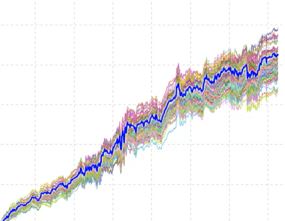
Note how concentrated the simulated equity curves are around the original backtest (bold blue line). Note also how the original backtest is centered within the simulated equity curves. In theory, both bode well for future performance.
Here is another good result:
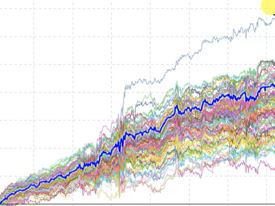
The simulated curves are more spread out, which translates to less confidence the strategy is actually fit to signal rather than overfit to noise. However, the outlier with windfall profits (on top) suggests a possibility that modulating noise can actually result in significantly better performance. The developers say this is a win and therefore a good result for the Noise Test.
Statistically speaking, I challenge this for two reasons. First, we have no idea whether this strategy is profitable going forward. Second, without a larger sample size I don’t know what to think about the profitable outlier. The Noise Test may be run on 10,000 different strategies without ever seeing this again. I can never draw meaningful conclusions from pure randomness.
The developers deem this a poor result of the Noise Test:
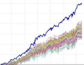
All simulated equity curves fare much worse than the original backtest, which suggests the original performance was fluke.
I will continue next time.
Categories: System Development | Comments (0) | PermalinkImplied Volatility Spikes
Posted by Mark on August 27, 2019 at 07:16 | Last modified: May 14, 2020 11:14One of my projects next year will be to clear out my drafts folder. Most of these entries are rough drafts or ideas for blog posts. This is one of 40+ drafts in the folder: a study on incidence of IV increase.
For equity trend-following (mean-reversion) traders, IV spike is a potential trigger to get short (long).
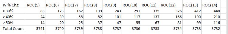
This was a spreadsheet study I did in December 2016. I looked at RUT IV from 1/2/2002 – 11/17/2016. I calculated the number of occurrences IV increased by 30% or more, 40% or more, and 50% or more over the previous 5 – 14 trading days.
Here are the raw data:
Here are the percentages:
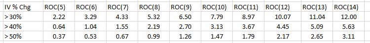
If I’m going to test a trade trigger, then I would prefer to find one with a large sample size of occurrences. Vendors are notorious for the fallacy of the well-chosen example (second-to-last paragraph here). This is a chart perfectly suited for the strategy, system, or whatever else they are trying to sell. When professionally presented, it looks wondrous; little do we know it represents a small sample size and is something that has rarely come to pass.
This trigger may avoid the small sample size categorization. Even in the >50% line (first table), periods of 8 – 14 show at least 30 occurrences. Some people regard 30 or more as constituting a sufficiently large sample size. I think length of time interval is relevant, too. We have roughly 15 years of data here. 30 occurrences is about twice per year. If I want four or more occurrences per year, then perhaps I look to >40% (period at least eight) or >30% as a trigger.
With regard to percentages, my mind goes straight to the 95% level of significance. Any trigger that occurs <5% of the time represents a significant event. I still don’t want too few occurrences, though. 1.5 standard deviations encompasses 87% of the population so maybe something that occurs less than 13% of the time or ~6.5% of the time (one-tailed) could be targeted.
Another consideration would be to look at the temporal distribution of these triggers. Ideally, I would like to see a smooth distribution with triggers spread evenly over time (e.g. every X months). A lumpy distribution where triggers are clustered around a handful of dates may be more reflective of the dreaded small sample size.
The next step for this research would be to study what happens when these triggers occur. Once the dependent variable is selected, we have enough data here to examine the surrounding parameter space (see previous link).
Categories: Backtesting | Comments (0) | Permalink