Backtester Logic (Part 8)
Posted by Mark on September 20, 2022 at 06:57 | Last modified: June 22, 2022 08:35Having tied up several loose ends in the last post, today I want to analyze logic for the find_short branch.
As with find_long (see here), find_short involves a multiple if statement:
![]()
The input variable (see key) from the top of the program is defined as follows:
width = int(input(“Enter spread width (in monthly expirations): “))
L98 searches for a DTE between upper and lower bounds. The difference between bounds is 10 days. The upper bound is the long option expiration minus (28 * width). With 28 or 35 days between expiration cycles, (28 * width) is the highest value it should ever take. The extra 10 [days] should accommodate a 35-day cycle.
If the width covers two (or more) 35-day cycles then this may not work because 7 * 2 = 14 days is more than the 10 provided. Moving the 10 inside parentheses won’t work because width = 4 (the least required to get two 35-day cycles) would allow for a lower bound that is ((4 * 28) + 40) below the upper bound: enough to capture two potential options for the short leg (although the desired longer-dated option will match first if the data file is complete).
To better code L98, I should include the additional days for each three months of width:
DTE > L_dte_orig – ((28 * width) + (10 * ((width + 2) // 3)))
Floor division ( // ) truncates the remainder for positive numbers. For one month, this is 3 // 3 = 1. For three months, this is
5 // 3 = 1. Only when I get to four months, which is 6 // 3 = 2, will 20 additional days be included.
I will make this modification, but for a couple reasons it’s not something I will use anytime soon. First, I really worry about liquidity and option availability for width > 3 because the long will then be very far from expiration and probably lightly traded. Practically speaking, I would only consider a max width of two months. Second, the lower bound seems unnecessary. Any option available in the long expiration should be available in the short as long as the data file is complete.*
If I want to clean the data files, which includes assessing completeness by searching for omitted and erroneous data, then I can create some simple Python scripts. That’s a topic for another post.
L99 looks to match strike price with the long option. One option per expiration cycle should match. I am okay with this line coming after L98 because the more restrictive if statement (see Part 4) may depend on how many expirations are available: a variable number over the years.
L99 also looks to match date with long option purchase. This is redundant because the previous if statement (not shown) checks for this and makes an entry in missing_s_s_p_dict if short not found.
I will continue next time.
*—This brings to mind another problem with 10-point multiples in find_long (see fourth paragraph Part 7).
Far from expiration, I have sometimes noticed that only 25-point strikes are available (and only 50-point
strikes going back many years). Requiring 10-multiple is actually constrained to 50-point strikes in that
case. The difference between one 50-point strike and the next can be much more than 1% of the
underlying in those earlier years, which is enough to make for a clearly directional trade.
Introduction to BetterInvesting
Posted by Mark on September 15, 2022 at 07:10 | Last modified: January 13, 2023 14:42I mentioned BetterInvesting in the last paragraph here. This is something I plan to use to help manage individual stock positions as part of a longer-term portfolio.
I subscribed to BetterInvesting late last year after finding the organization in fall 2021. From their website:
> Today NAIC [National Association of Investment Clubs] is known as BetterInvesting, a 501(c) (3)
> nonprofit association that remains dedicated to helping individuals and investment clubs learn and
> practice our fundamental approach to stock investing. Passionate volunteers, who follow our
> principles and practice the SSG [Stock Selection Guide], teach our educational programs. The SSG
> is available online 24/7, making it even easier to study and invest in stocks.
I don’t think of it like a service to be sold as much as I do a tool for analyzing stocks. Their approach covers a wide breadth and if someone is going to do fundamental analysis to any degree, then something to organize all the inputs and a process guiding what to do with them can be extremely valuable. One could do without such a tool and if this is something you try, then I’d be interested to hear what you do to get all the information and just how long it takes.
Personally, learning the BetterInvesting approach has given me a process to gather relevant data and make investment decisions in 1-2 hours per stock. Prior to this, I really had no idea. If I wanted to make decisions based on fundamental analysis, then I could look at suggested buy lists, perhaps investment newsletters (which I think are generally a waste of money), and some other places.
In 2001, I developed a stock screen after some book reading that was effectively the beginning to managing my own portfolio. It took me about an hour per week and I fared well with it on an absolute basis. I never revisited this once I discovered options in 2006. While I’ve thought about rekindling the original stock screening effort in recent years, I have also become a true believer in classic fundamental analysis for longer-term purposes. This is more the BetterInvesting way.
Any explanatory content I publish under the category BetterInvesting might be better studied in the video education library on their website since I’m a new member rather than an official instructor or volunteer. I might actually like to become a volunteer if it got me out to the community to teach the process to other like-minded individuals.
This would then beg the question whether their process is the best? I think we’re far away from having enough information to answer that question with any validity. I believe having a process and sticking with something repeatable to optimize efficiency is probably as good as anything else.
Categories: BetterInvesting® | Comments (0) | PermalinkBacktester Logic (Part 7)
Posted by Mark on September 12, 2022 at 06:54 | Last modified: June 22, 2022 08:35Today, I want to tie up some loose ends related to multiple topics.
The issue of trading options farther out in time (see paragraphs 3-4 of Part 6) will resurface later when I discuss time spread width. For now it will suffice to say that if I want to increase width, besides trading a longer-dated long option I can also do a shorter-dated short option when slippage (open interest, volume, liquidity, etc.) is a concern.
L71 (see Part 4) filters for a 10-point strike by requiring the remainder of strike price / 10 = 0. Due to liquidity concerns, I would prefer to trade only 25-point strikes. My second choice would be 10-, and 5-point strikes would be last. I don’t have actual execution data to support this—it’s just gut feeling based on what I’ve anecdotally heard from other traders.
One potential issue with filtering for strike multiple is a strike density decrease with lower price of the underlying. The relative difference between one 10-point strike and another generally gets larger going back in time where SPX is valued lower. With SPX at 4000, 10 points is only 0.25%. With SPX at 1500, though, 10 points is 0.67%. I cannot say how significant a concern this is, but it would be 2.5x worse for 25-point strikes. The base strategy is not intended to be directional.
Going back to L70, I no longer need the lower bound with my proposed solution in the second paragraph of Part 6. The program will find the first option that has less than (((mte + 1) * 30 ) + 5) DTE. The extra five along with 30 (two more than the more common 28-day) will cover a 35-day expiration cycle, which happens once per quarter. The option I want will be that or the next-lower DTE option to match. The latter will be checked by the check_second flag.
Rather than nested ifs, I could code as an if-else block per fifth paragraph of Part 4, but I don’t see any real advantage. Additional logic in the else block may dictate that nothing be executed for the current iteration (only 0.4% of rows are used). I would have to include a pass (null) statement or two (as if-elif-else) since if-else forces execution of one branch or the other.
In the second paragraph of Part 4, I said the update_long logic avoids a subsequent match to options on the same date even though the same-date options are not being skipped. That logic is in L134:
![]()
This looks to match strike price and expiration date. Recall the third paragraph here. Once find_short is complete, same-date options are avoided despite the wait_until_next_day flag being circumvented because each strike/expiration combination only appears once per historical date. Is this more or less efficient?
Although I may be wrong due to “mitigating factors” (second-to-last paragraph of Part 4), I would hypothesize matching strike price and expiration date to be less efficient than skipping dates with wait_until_next_day. The latter requires one truth test to compare current_date and historical date whereas update_long’s and statement requires two.
Loose ends be gone!
Categories: Python | Comments (0) | PermalinkBack from the Hack
Posted by Mark on September 9, 2022 at 06:37 | Last modified: January 13, 2023 13:52My apologies for any “404 error” you may have gotten recently when trying to navigate my website. The site was hacked by malware. I don’t know if it was down for days, for weeks, or for months. I subscribed to a security package and have been told that everything is now restored.
2022 has been a tough time for trading: my most difficult since beginning full-time in [and including] 2008. This year has left me staggered and raw. It’s attacked my positivity and hope. I will blog more about this in coming posts.
Despite the hit, I’m not ready to give up yet. Throwing out the baby with the bathwater is never a good idea and to that end, I still have work to do.
The Python backtester is on life support. You will continue to see posts on Python work I did earlier this year. For me, the dagger was realization that the data and corresponding results were irrevocably compromised.
While I haven’t practiced Python for several months, the next time I revisit will be my fourth “tour of duty.” I got farther the second time in 2020 than I did the first (2019). The third (2021-2022) was mostly practical application in working with the backtester. Hopefully the fourth comes easier and allows me to reach greater depths. Backtester aside, I have other projects in mind for which programming may be useful. Stay tuned for additional blog posts in the Python category.
Thankfully, some new automated backtesters have come onto the market. I have taken a good look at Option Omega, which has many appealing features. I also recently learned about MesoSim, which may be more tailored to my kind of trading.
I’m not really sure whether subscribing to one of these services solves the data issue. It’s at least likely to hide data flaws because close scrutiny of the backtrade log will be required. Making matters worse, some automated backtesters don’t provide such a log with essential data like entry and exit prices. This would allow for verification especially when trade results are highly discrepant from anything seen in ONE where the complete option chain is on display.
Either way, I have not entirely given up on backtesting and still have option strategies I’d like to study with an automated product. I will blog about this in the near future.
Something I have discovered in the past several months is BetterInvesting, which focuses on technamental [see Take Stock by Ellis Traub (2010)] analysis of stocks. Most important to me in this pursuit would be a repeatable process, which BetterInvesting provides. I don’t care so much what the process is because testing/validating the process would require [backtesting] tools that I’m not even sure exist. Regardless, you can expect some future blog posts in this area under the new category tag “BetterInvesting.”
Categories: About Me | Comments (0) | PermalinkBacktester Logic (Part 6)
Posted by Mark on September 6, 2022 at 06:45 | Last modified: June 22, 2022 08:35Today I want to finish ironing out the logic from L70 shown here then continue to analyze that conditional skeleton.
As an example of my proposed solution at the end of Part 5, in 2015 (date 16448) we have options with 94 DTE followed by options with 66 DTE. Both pass L70, which means the latter is what I want. I can add a Boolean flag check_second that starts out as False. Once int(float(stats[2])) no longer equals L_dte_orig (see key), the flag gets changed to True. If this passes L70 then find_long continues in this DTE. If it fails L70, then change control_flag to find_short and continue (to the next iteration) without setting wait_until_next_day to True.
In addition to the 60 – 95 DTE range, I am also interested in studying longer-dated time spreads despite potential issues with slippage. Examples include 90 – 125, 120 – 155, and 150 – 185 DTE. Live trading is the best way to understand slippage. Unfortunately, I can’t go back and live trade in previous years. Common wisdom suggests slippage will be lower with higher volume and open interest, but the data files don’t allow me to test this. I could plot volume and open interest over time, but this may be a waste of time since I have no way to know how that might translate to slippage.
Another thing that may limit my ability to backtest longer-dated options is historical availability. Over the years, more expirations and more strike prices have come available coincident [I suspect] with higher-volume option trading. In 2015, 168 DTE is available followed by 105 DTE, which means I can’t do a time spread one month wide. Things change in 2020. In early Jan 2015, monthly expirations appear for the first four months. In early Jan 2020, monthly expirations appear for the first six months. This expresses my concern despite being anecdotal observation.
One thing I don’t see in the conditional skeleton is a continue statement at the bottom. Whether or not the backtester identifies the current row as the long option, it can then advance to the next iteration (row). Without a continue statement, the program will go on to unnecessarily evaluate control_flag three more times before advancing. “Continue” should conclude the first three branches. Completing the block, the last branch doesn’t need a continue statement as advancing to the next iteration will automatically take place.*
I will press forward next time.
*—Actually, I did remember this. The Atom text editor features folding to hide blocks of code as described
here. With “continue” being the last line of the previously indented blocks, they were hidden.
Time Spread Backtesting 2022 Q1 (Part 9)
Posted by Mark on September 1, 2022 at 06:49 | Last modified: May 18, 2022 17:16Today I will conclude my time spread backtesting for 2022 Q1.
I left off at the second adjustment point of trade #14. Pre-adjustment, this is very close to max loss.
Whether the mere act of adjusting makes ROI% better or worse is simply a matter of arithmetic. The first adjustment worsens ROI% from -7.4% to -8.1%. The second adjustment improves ROI%. MR increases by $1,388, which is a bigger change than that resulting from the first adjustment (+$568). PnL pre-second-adjustment is -19% vs. -7.4% for the first, though. To maintain ROI%, the larger MR would have to be accompanied by a loss that is $263 higher. Transaction costs are fixed at $21/contract, which is $84/adjustment. Because $84 < $263, the second adjustment dilutes ROI% back to -16.8%:
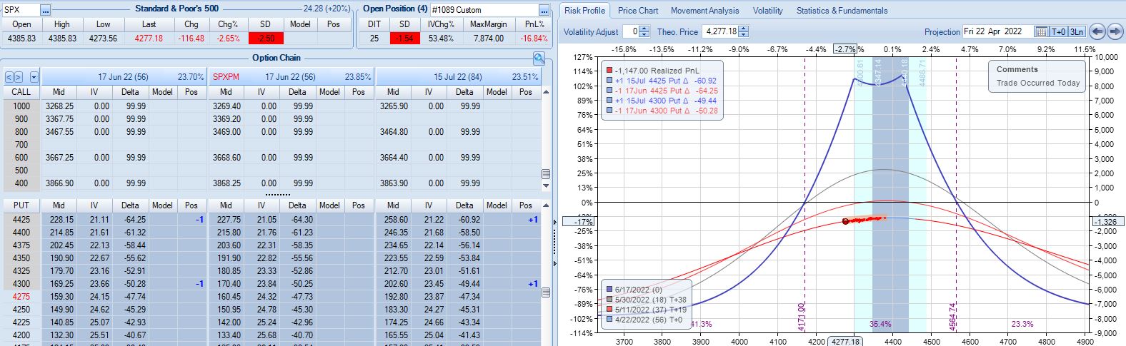
At this point, TD = 11. According to ONE, I only have ~1% of downside before -20% max loss is reached.* Is the adjustment worth doing? Certainly in the absence of a guideline preventing it (see base strategy in Part 1), I have to say yes.
Max loss is hit at -21.4% four days later on a 2.12 SD market decline. For the trade, SPX falls 1.88 SD over 29 days although it’s only down 1.34 SD over 28. Unpredictability of large moves is one reason this endeavor can be so difficult.
In total for 13 trades entered in Q1,** the base time spread strategy makes $1,855 on a max margin of $10,252. The latter also represents the greatest increase from initial capital (+45%) seen in 158 historical trades. Although it’s probably far more than I need, I like to err on the side of conservatism. Doubling the $10,252 will provide for a substantial margin of safety.
The time spread return is therefore +9.0% for Q1 2022 compared to -12.8% for SPX. That is a shellacking with which I would be quite satisfied (compare here). The overall PF is low (but profitable!) at 1.28. The average win (loss) is $938 (-$1,647) on 9 (4) total wins (losses). Over just 13 trades, the max consecutive number of wins vs. losses is two vs. eight, respectively: pretty healthy [for equity curve to hang out near all-time highs most of the time]. Those two started out the year, though, which made for what would ultimately be the max drawdown (MDD) of -15.7%.
Rounding up to four total months of backtesting, the annualized time spread return is +27%. As always, don’t count on any good result repeating every year.
Taking a normalization approach, MR for each trade can be divided into any fixed number you choose to get position size. The PnL numbers then turn out slightly different. Normalizing for $100K, I get a Net PnL of $21,541 (+21.5%) and a PF of 1.21, which is slightly worse than without normalizing (heed the less-impressive result). MDD after the first two trades is about -49%. That’s way too high for my risk tolerance. MDD would be -19.6% if normalized for $250K MR. I find this more reasonable. At this level, total return falls to +8.6%, which is +25.8% annualized.
* — The automated backtester would not have access to this information.
** — 14 includes trade #3 starting 3/9/22 and trade #11 starting 3/7/22. I took the worst
of the two since both occurred in the same week.
Backtester Logic (Part 5)
Posted by Mark on August 29, 2022 at 07:14 | Last modified: June 22, 2022 08:34Today I continue to dissect the conditional skeleton of the find_long branch shown near the bottom of Part 4.
L70 – L72 includes eight data type conversions. Early on, I was frustrated with unnecessary decimal output. To fix this, I tried converting applicable fields to data type ‘int'[eger] and some resulted in an error. Doing int(float()) was a successful workaround. I should revisit to see if the readability of output is improved enough to justify the added processing. For curiosity’s sake, I can add a timer to the program and check speed.
L70 filters options by DTE. I can make this more readable by creating two variables for lower and upper bounds followed by one if statement that calls for the variable to fall in between.
As mentioned above, I could add a timer to the program to see if this helps, but I don’t want to get bogged down with repetitive time measurements. If the backtester works, then I’m fine whether it takes 10 minutes 34 seconds or 12 minutes 28 seconds. Either way, I’ll be happy to get the results and spend the bulk of my efforts analyzing those.
Before the program calls for iterating through the data files, I have:
> mte = int(input(‘Enter minimum (>= 2) months (1 mo = 30 days) to long option expiration: ‘))
Suppose I enter 2. At L70, the backtester will search for > 2 * 30 = 60 DTE. This is clear as the lower bound.
The upper bound is more complex because every quarter we get five weeks between consecutive expiration months rather than four. 92 DTE will meet the criteria and be correct only when 92 – 28 = 64 DTE does not follow in the current expiration. Data files are organized from highest to lowest DTE (see Part 1). With the goal to maximize efficiency by having the backtester going through the files once, I can’t have it iterating down and then having to go back up if what it finds below is not a match.
Thankfully, it doesn’t have to be that complicated.
The solution is to select and encode the first passing option but wait to leave the find_long branch until DTE changes. The program can then test whether the subsequent DTE also meets the criteria. If so, dump the values from the former and search for a new match. Otherwise, use the former. Switch to the find_short branch once this is all done.
If the first option meeting the criteria is less than 60 + 28 = 88 DTE, then no circumstance exists where the next DTE to appear will pass. In that case, no second check is even needed.
I will continue next time.
Categories: Python | Comments (0) | PermalinkLessons on Twinx()
Posted by Mark on August 26, 2022 at 06:48 | Last modified: May 17, 2022 15:57I spent the whole day yesterday trying to figure out why I got overlapping axis labels on a secondary axis for my graph. I want to document what I’ve learned about the twinx() function.
Let’s start by creating a df:
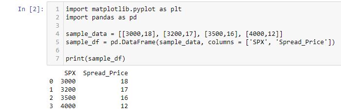
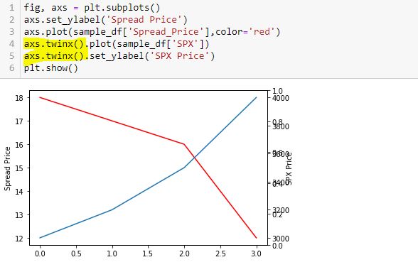
Now, I’m going to add two lines. Spread price will be in red and SPX price will be in blue:
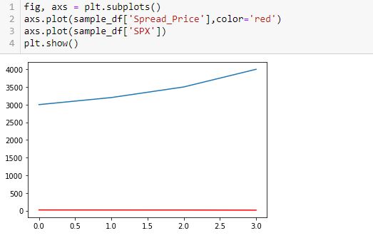
This doesn’t work very well. In order for the y-axis to accommodate both, the spread price looks horizontal since its changes are so small relative to the magnitude of SPX price.
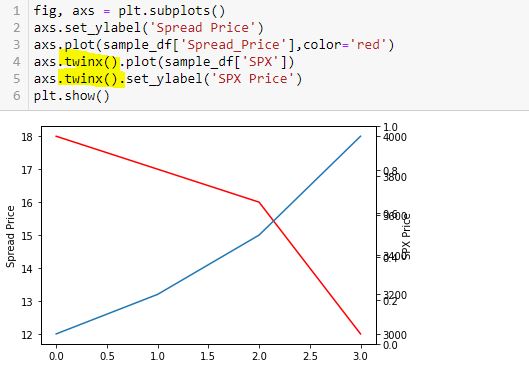
To fix this, I will create a secondary y-axis on the right side:
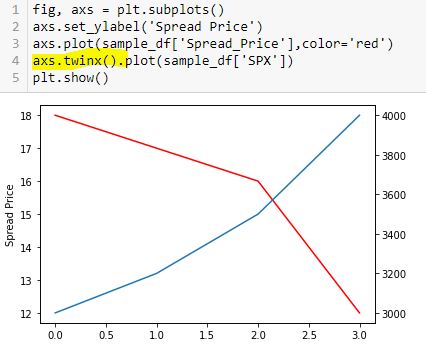
Now, I label the right y-axis:
Whoa! This generates an overlapping set of y-axis labels on the right going from 0.0 to 1.0. What happened?
Here is a correct way to do this:
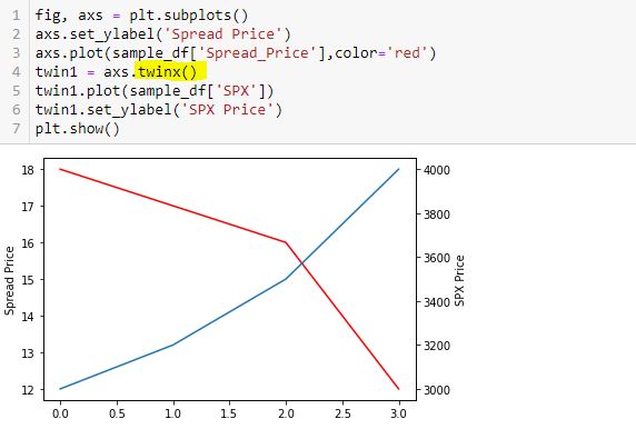
Thinking substitution is what confused me. I saw this solution online but got confused because I interpreted L5-L6 as substitution from L4 and had trouble wrapping my mind around it. I therefore chose to do it the long way:
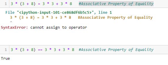
This is not the way Python works. Python is not algebra.
Had I questioned this [which I didn’t], I could have verified with a truth test:
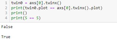
L2 is False (unlike L4, which is obviously True).
twinx() creates a new y-axis each time it is called. Calling more than two can lead to the overlapping labels.
Furthermore, a function or method like twinx gets called each time the function/method name is followed by (). When you see “name()”, you are seeing a function/method call. This is not something I ever read in documentation or in Python articles. To me, this most definitely is not obvious. The third and fourth code snippet above include twinx() once and twice, respectively. This is why the fourth has an overlapping y-axis. The fifth code snippet has twinx() just once: no problem.
Anytime I see a single equals sign, it might help to think “is assigned to.” The variable will retain said value until something dictates otherwise. No substitution is taking place and no properties of equality necessarily apply.
Once more for emphasis:
Backtester Logic (Part 4)
Posted by Mark on August 23, 2022 at 06:34 | Last modified: June 22, 2022 08:34I left off tracing the logic of current_date through the backtesting program to better understand its mechanics. The question at hand: how much of a problem is it that current_date is not assigned in the find_short branch?
Assignment of control_flag (see key) to update_long just before the second conditional block of find_short concludes with a continue statement is our savior. Although rows with the same historical date will not be skipped, the update_long logic prevents any of them from being encoded. Unfortunately, while acceptable as written, this may not be as efficient as using current_date. I will discuss both of these factors later.
The update_long branch is relatively brief, but it does assign historical date to current_date thereby allowing the wait_until_next_day flag to work properly.
Like find_short, the update_short branch begins by checking to see if historical date differs from trade_date. I coded for an exception to be raised in this case because it should only occur when one leg of the spread has not been detected—preumably due to a flawed (incomplete) data file. Also like find_short, update_short has two conditional blocks. At the end of the second block, wait_until_next_day is set to True. This can work because current_date was updated (prevous paragraph).
I have given some thought as to whether the two if blocks can be written as if-elif or if-else. In order to answer this, I need to take a closer look at the conditionals.
Here is the conditional skeleton of the find_long branch:

Right off the bat, I see that L71 is duplicated in L72. I’ll remove one.
Going from most to least restrictive may be the most efficient way to do these nested conditionals. In the fourth-to-last paragraph here, I discussed usage of only 0.4% total rows in the data file. Consider the following hypothetical example:
- Data file has 1,000 rows of which 4 (0.4%) will ultimately be used.
- 50, 100, and 200 rows meet the A, B, and C criteria, respectively.
- Compare nested conditionals “if A then if B then if C…” (Case 1) vs. “If C then if B then if A…” (Case 2).
- All 1,000 rows get evaluated by each Case.
- Case 1 leaves only 50 rows to be evaluated after the first truth test vs. 200 for Case 2 and Case 2 likely has more rows still left to be evaluated going into the final truth test.
- Case 1 is more efficient.
All else being equal, this makes sense to me.
Other mitigating factors may exist, though, like number of variables involved in the evaluation, data types, etc. In trying to apply this rationale to the code snippet above, I may be overthinking something that I can’t fully understand at this point in my Python journey.
I will continue next time.
Categories: Python | Comments (0) | PermalinkTime Spread Backtesting 2022 Q1 (Part 8)
Posted by Mark on August 18, 2022 at 06:40 | Last modified: May 18, 2022 14:17I will begin today by finishing up the backtesting of trade #12 from 3/14/22.
The next day is 21 DTE when I am forced to exit for a loss of 16.5%. Over 46 days, SPX is down only -0.09 SD, which is surely frustrating as a sideways market should be a perfect scenario to profit with this strategy. I am denied by an outsized (2.91 SD) move on the final trading day. Being down a reasonable amount only to be stuck with max loss at the last possible moment will leave an emotional scar. If I can’t handle that, then I really need to consider the preventative guideline from the second-to-last paragraph of Part 7 because the most important thing of all is staying in the game to enter the next trade.
One other thing I notice with regard to trade #12’s third adjustment is margin expansion. The later the adjustment, the more expensive it will be. As I try to err on the side of conservativism, position sizing is based on the largest margin requirement (MR) seen in any trade (see second-to-last paragraph here) plus a fudge factor (second paragraph here) since I assume the worst is always to come. This third adjustment—in the final week of the trade—increases MR from $7,964 to $10,252: an increase of about 29%! The first two adjustments combined only increased MR by 13%.
The drastic MR expansion will dilute results for the entire backtest/strategy, which makes it somewhat contentious. To be safe, I would calculate backtesting results on 2x largest MR ever seen. If I position size as a fixed percentage of account value (allows for compounding), then I would position size based on a % margin expansion from initial. For example, if the greatest historical MR expansion ever seen was 30%, then maybe I prepare for 60% when entering the trade.
With SPX at 4454, trade #13 begins on 3/21/22 at the 4475 strike for $6,888: TD 23, IV 20.0%, horizontal skew -0.4%, NPV 304, and theta 39.
Profit target is hit 15 days later with trade up 11.8% and TD 21. After such a complex trade #12, this one is easy.
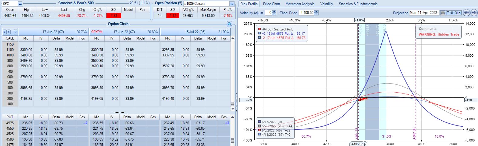
With SPX at 4568, trade #14 begins on 3/28/22 at the 4575 strike for $5,918: TD 25, IV 15.8%, horizontal skew -0.4%, NPV 274, and theta 24.
On 67 DTE with SPX down 1.81 SD, the first adjustment point is reached:
On 56 DTE, SPX is down 2.50 SD and the second adjustment point is hit:
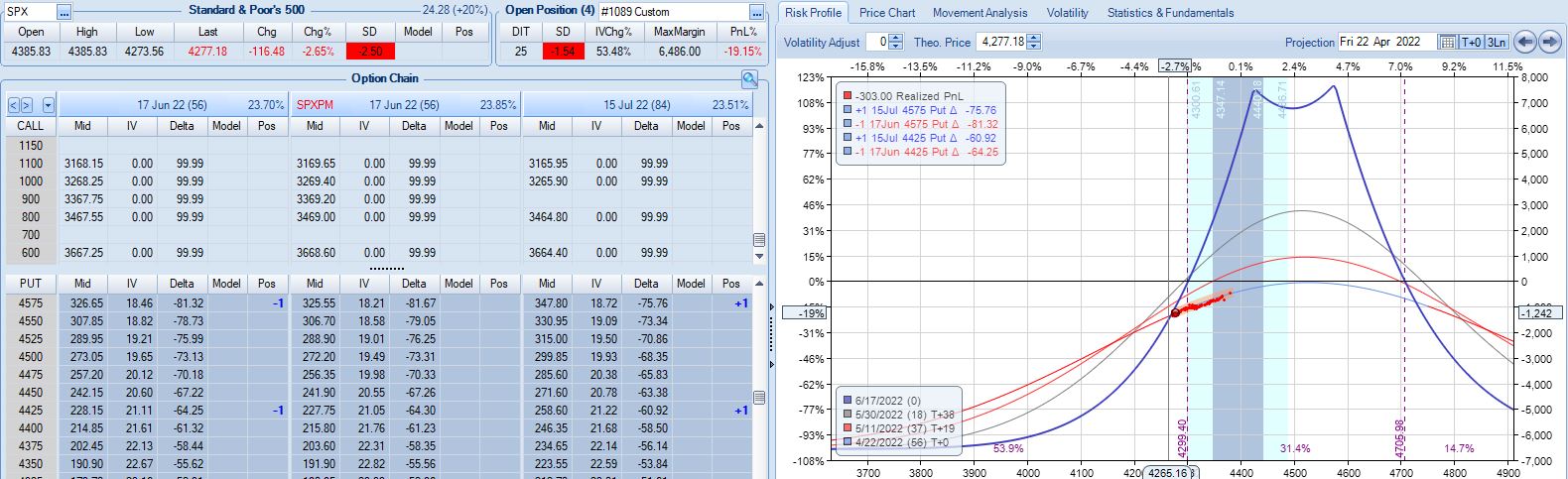
Despite being down no more than 10% before, the trade is now down 19.2% after this huge move. With regard to adjustment, I’m now up against max loss as discussed in the fourth paragraph of Part 6.
I will continue next time.
Categories: Backtesting | Comments (0) | Permalink