Naked Call Backtest (Part 3)

Before proceeding with more backtesting data, I want to clarify some previous points and make a casual observation.

Position sizing based on max drawdown (DD) says “the largest DD I ever saw in backtesting was X. If I never want more than a Y% DD on my account, then minimum account size is X / (Y / 100).” As an additional margin of safety, suppose the largest future DD will exceed max DD by a factor of Z. The minimum account size becomes (X * Z) / (Y / 100).

Given the $407K MDD (one contract initial size), preference not to see my account down more than 20%, and anticipation of future max DD 2x worse than that seen in the past, minimum account size should be ($407K * 2) / (20 / 100) = $4.07M.

Even if I can position size this way based on max DD, portfolio margin requirements (PMR) could still be a limitation. As account equity decreases and margin limits approach, I may not be able to continue holding the position. Recall from Part 1 that depending on index value, PMR is $1.7M – $3.3M when starting with one contract. A $4.09M account suffering a 40% DD becomes $2.45M, which can no longer support a $3.3M PMR.

DD and position size both determine whether an account can support a position. Position size is proportional to PMR. DD affects buying power. A margin call will be issued by the brokerage as buying power approaches [and certainly slips below] PMR forcing clients to deposit additional funds or to close positions (else the brokerage will do so for them).

Vertical spreads cap PMR, which is still proportional to index price. We probably need to determine the larger of max PM or max DD (along with associated fudge factors discussed in second paragraph) and base position sizing off that.

Large variance across IV and index price level demands more dynamic guidelines for normalization. This backtest implements a static premium in the face of wide-ranging underlying price and volatility. Implementing a static delta, instead, would allow for a normalized strategy that proportionally self-adjusts over time.* If I were doing spreads, then width could be better defined [dynamically] in terms of index price since a static 200 points is 10% of 2000 and only 5% of 4000.

This can all be confusing, which is why I wrote an entire mini-series on it.

As a final note, this backtest closes all short options no later than 3:50 PM on expiration Thursday. In live trading, the short option can often be left to expire thereby saving premium and transaction fee. A cursory review of current results reveals a difference up to $15K: sizeable, to be sure, but amounting to little more than a rounding error all things considered.

*—Added to my to-do list.

Naked Call Backtest (Part 2)

I left off analyzing naked calls with respect to portfolio margin (PM) and maximum drawdown (MDD).

The strategy could be implemented based on maximum drawdown (MDD), but margin is another clear limitation. Even one contract could require up to $3.3M in PM for ~$108K profit. This paltry 0.34% total return gets even smaller as the index continues to climb. Not worth it!

One thing I could do to decrease PM would be to sell the vertical spread instead of naked call. Going 200 points wide would risk up to $20K/contract. Ten contracts would be up to $200K in PM, but I certainly could not increase 64-fold from there.

The spread concept brings with it some other interesting revelations. The backtest starts in high IV:

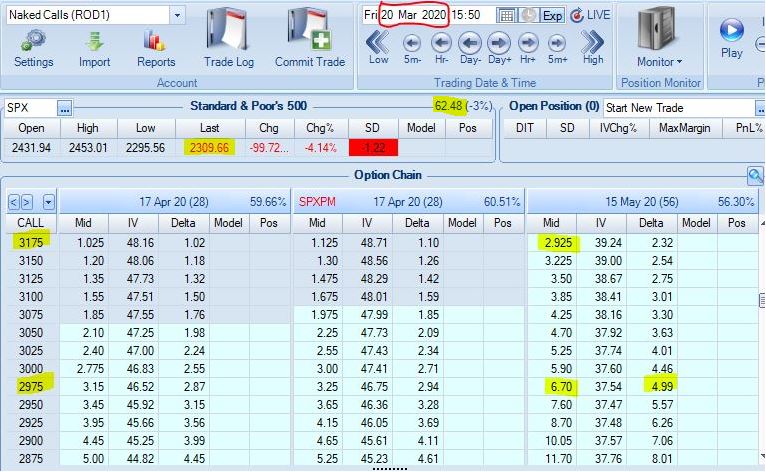
Observations:

• 200 points wide, which is $20K/contract risk
• Net credit ~$3.75 (~$4.40 going one strike NTM)
• Well into second standard deviation (SD) OTM
• Short delta ~5 (~5.6)

The backtest ends in low IV:

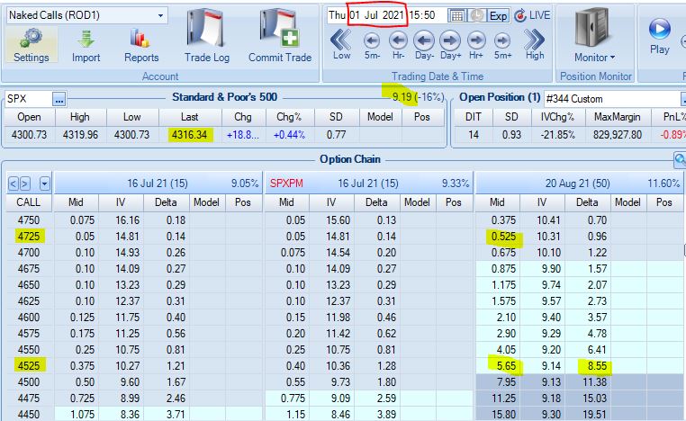
Observations:

• 200 points wide, which is $20K/contract risk
• Net credit just over $5.00 ($7.25 going one strike NTM)
• Just barely into second SD OTM (last strike in first SD OTM)
• Short delta ~8.6 (~11.4)

High IV is lower risk in terms of delta, but generates less credit because the long option is relatively expensive compared to the short. Low IV collects more credit but does so at a relatively higher delta, which is more risky.*

These examples illustrate two major differences: IV and index price. With regard to the latter, selling a fixed dollar amount is relatively NTM (higher delta) for index at lower value compared to relatively OTM (higher delta) for index at higher value.

To see what SPX around 2300 would look like in low IV, we can go back to 12/23/16:

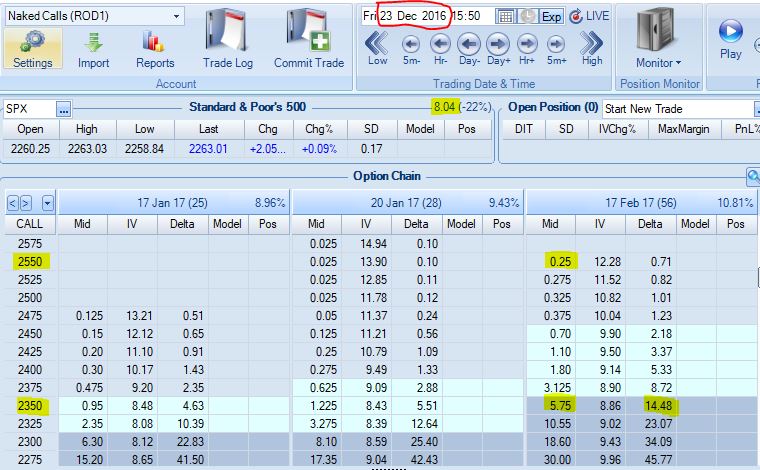
Observations:

• 200 points wide, which is $20K/contract risk
• Net credit $5.50 (~$2.90 going one strike OTM)
• Last strike within first SD OTM (just into second SD)
• Short delta 14.5 (8.7)

The first two examples suggest higher IV may hurt credit, but now we see that lower IV also results in lower credit if sold at a comparable delta value.

Also note that I can cut risk 50% by purchasing the long leg 100 points NTM for only $0.45 more.

I will continue next time.

* — I have discussed two different kinds of risk here. Spread width defines risk as the maximum
       loss for any given trade. Delta represents risk by approximating probability of expiring OTM
       (full profit) as opposed to ITM (likelihood of loss).

Naked Call Backtest (Part 1)

For the last several years, I have not been a proponent of selling naked calls. However, “necessity is the mother of invention.” Volatility does not explode to the upside; how bad can they actually be?

Here are my backtesting guidelines:

• Use OptionNet Explorer (ONE) between 3/23/2020 – 7/1/2021.
• Sell 10 naked calls in monthly expiration closest to 30 DTE for ~$7/contract.
• Use 25-point strikes only.
• Assess transaction fee of $16/contract (slippage and commission).
• Monitor market once daily at 3:50 PM ET.
• If ITM, roll to following month as far OTM as possible for credit and double size.
• Otherwise, rinse and repeat on expiration day.

This is the backtesting period:

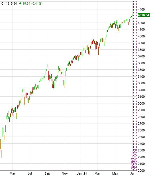
To understand how bad naked calls can possibly be, this seems to be a pretty good place to start. SPX 2254 to 4316 is an increase of ~91% in just over 15 months: a staggering [recovery and] ascent! I expect to see losses under these conditions.

Here are the overall results:

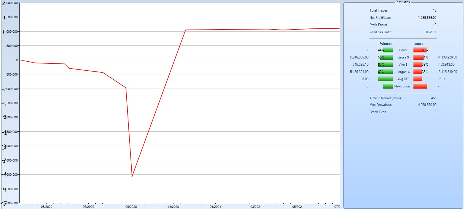
This is a strange looking equity curve. It certainly does not match my ideal, which would be upward sloping at 45 degrees. From inception through Sep 2020, this strategy does a wonderful job losing money. From Nov 2020 on, it looks flat. In between the two periods, it makes a ton of money.

Trade statistics indicate this strategy loses more often than it wins and that the average winner is bigger than the average loser. Overall, this shakes out to a profit factor of 1.3.

Take it or leave it?

Let’s look closer to the individual trade results:

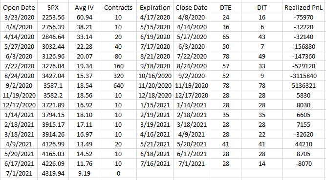
The first seven trades are all losses and position size doubles each time. No wonder the numbers on the equity curve get huge. A win finally recoups all losses and then some. Position size remains comparatively low for the remainder of the backtest (10-20 contracts compared to the high of 640), which is why the curve is flat on the right side.

One trade out of 16 saves our bacon.

Actually, what saves our bacon is not the particular trade but rather the position size. Any of the winning trades sized at 640 contracts would generate enough profit to overcome the losses.

We must not forget about risk. Portfolio margin (PM) for naked calls is 12%. With SPX at 2254, this amounts to 2254 * 100 * 0.12 = $27,048/contract. With SPX at 4316, this amounts to 4316 * 100 * 0.12 = $51,792/contract. The initial position size carries a PM requirement between ~$270K – $518K. 640 contracts carries a PM requirement between ~$17M – $33M where
M = million. This backtest includes a 64-fold increase in position size!

At this point, I have to say leave it. Even with one contract, PM requirements are too large and the MDD ($406K) is too big.

I will continue next time.

Put Diagonal Backtest (Part 6)

I spent time backtesting yesterday and wanted to make a couple comments before presenting additional data.

First, I did ask my brokerage about this footnote:

      > I’m thinking about selling a weekly SPX ITM put and rolling this as a
      > campaign. However, rather than close out the expiring SPX ITM put, I
      > would just let it get assigned and open the next one. I want to make
      > sure this will not incur any fees aside from debiting my account for
      > the intrinsic value of the option at expiration.
      >
      > Can you confirm this?

They responded:

      > SPX is cash settled so you would just see a cash credit or debit
      > based on the settlement value. There are no commissions/fees for
      > exercise/assignment.

This implies I may have overcompensated for slippage as discussed in Part 1. I like to err on the side of caution. Since backtesting has a tendency to artificially inflate results, decisions should be based on conservative projections.

Taking assignment on short options is beneficial. Not only does it allow me to retain maximal extrinsic value, which goes to zero at expiration, it also saves me transaction fees on the buy-to-close.

The potential downside to taking assignment is legging risk. Bid/ask spreads widen at 4:00 PM (normal close) and beyond as mentioned by OptionNet Explorer (ONE) support here. To avoid the wider spreads, I would open the new short position after 3:50 PM knowing the old will expire 25 minutes later. Legging risk refers to the possibility I may lose money due to an underlying price decline. Had I waited until 4:15 PM to open the new short, I would have avoided unrealized loss.

The backtest avoids legging risk by rolling to ensure concomitant execution of both options. “Trade like you backtest” has therefore been violated, which signifies the presence of backtesting inaccuracy.

Legging risk introduces backtesting uncertainty due to data limitations. Because ONE data stops at 3:55 PM, I cannot measure what happens through the 4:15 PM expiration. Over a large sample size, I would expect any gains and losses to average out since I don’t believe any edge exists by consistently going long or short equities from 3:55 PM to 4:15 PM.* Too bad the put diagonal backtest does not encompass a large sample size.

Another source of uncertainty is the remaining extrinsic value I pay to close short options in ONE. I used either 3:30 PM or 3:55 PM in the backtest. Shame on me for not being cognizant and consistently using the latter since time decay accelerates in the last 25 minutes: 3:30 PM includes more extrinsic value than 3:55 PM. This paid extrinsic value represents additional expense that would not exist in live trading, and uncertainty exists because I failed to measure it.

I will conclude next time.

* — This can be tested (make sure to factor in transaction costs).

Put Diagonal Backtest (Part 5)

Just to reiterate, the goal is to stay as far OTM as possible to collect all intrinsic value made available. I will collect the intrinsic value regardless of when I roll unless the market overruns, in which case I start to lose intrinsic value because rolling up will go toward capturing extrinsic until short strike is above the underlying price.

The temptation when DITM with very little extrinsic value being collected is to roll down. Watch out, though, because being overrun can cost us dearly.

The following research question remains: is it more efficient to maintain constant strike price over a series of rolls or can I do just as well if it fluctuates (lower, higher, lower, higher, etc.) within ITM range? If the former is true, then keeping strike price constant and taking the slippage hit (third-to-last paragraph here) would be more plausible. I will backtest this.

As mentioned in this second paragraph, the occasional overrun cannot be avoided. To avoid overruns at all costs, I would have to sell sufficiently DITM that TEV would rarely be attained.

That same sentence implies LIVOC can be recouped by selling additional EV later. As mentioned in Part 2 paragraph 3, amortizing this over the remaining LP life is prudent. I don’t plan to hold LP to expiration due to accelerated time decay. Taking this into consideration along with the up-and-out roll when market rallies 5-10%, perhaps amortization should be done only over the actual duration I hold the LP. This would have to be a retrospective calculation, which means any leftover deficit could be added to the subsequent LP TEV.

How bad can the overrun losses really be? Look at the risk graph below:

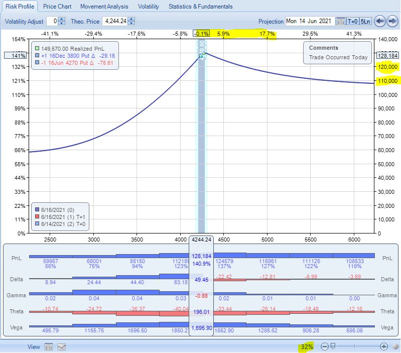
The upside looks pretty dangerous! The highlighted numbers on the right suggest I can lose $10,000 pretty quick, which would be a chunk of the profit accrued to date.

Looking across the top, though, reveals these to be huge changes in the underlying. I should zoom in (note percentage at bottom right) and focus over a more reasonable amount of underlying movement for the next few expirations:

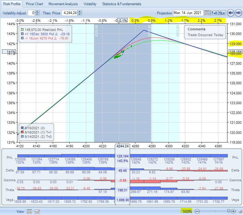
Now I see that even from the peak, I would lose only ~$1,000 on a 3% upside move. This is not catastrophic loss. Let’s keep this in mind before thinking the worst, which I suggested as the “double whammy” in the fifth paragraph of Part 4.

One final backtesting note: on weeks when monthly options expire, be sure to use SPXPM because the monthly expires Friday morning and we don’t want to contend with settlement risk.

Put Diagonal Backtest (Part 4)

Today I continue with discussion and analysis of my first ever put diagonal backtest.

I left off saying once my short option goes OTM, the only way I can recoup the loss is if the market subsequently crosses below my strike. Once I roll when OTM, intrinsic value is lost…

…for good?

Suppose I roll out to the same strike, market reverses lower, and the option is again ITM at expiration. The LIVOC has now been restored. This is a gamble because equities historically display positive drift by rising more than 50% of the time. The risk is that a small amount of LIVOC becomes a huge amount of LIVOC if the market continues to rally.

Rolling straight out on Mar 23, 2020, for example, could be devastating. This is one of many up days at the start of a huge uptrend covering hundreds of points. Compounding positional losses with the reality of losing big while everyone else is gaining/winning amounts to a double whammy from which psychological recovery could prove extremely difficult. This is directly related to the subject of emotional investing.

If the market seems to be in a downtrend, then I can gamble by rolling OTM rather than ITM. If correct, then I avoid losses that would otherwise result from increased intrinsic value down to the strike price: when intrinsic value starts to build. Again, I call this gambling for the same reason given two paragraphs above.

The struggle is real between rolling to a lower strike and rolling to the same DITM strike for no extrinsic value and potential loss due to slippage. As the market falls and I remain on the fringe of TEV or less, I am tempted to roll down to be more within the meat of the T. Prem distribution (displayed in the second table of Part 3). This would raise more than TEV and prevent me from facing this dilemma repeatedly over subsequent expirations.

In the backtest, I sometimes rolled out 2-3 weekly expirations (4-7 additional days) to capture what seemed like a reasonable average EV. As an example, sometimes rolling out 3 DTE—Friday to Monday—would generate zero EV but 5 DTE—Friday to Wednesday—could be done for $2.20 EV, which is an average of $1.10 over two cycles. If my TEV were $1.00, then I would take that! I hate to lose money due to slippage alone, which argues for rolling down and collecting enough EV to offset.

I would still have to roll higher for the subsequent expiration after a big up day, though, and this represents LIVOC risk.

I will continue next time.

Put Diagonal Backtest (Part 3)

Today I want to explore roll mechanics and discuss when might be the best time to roll in order to avoid LIVOC (defined here).

The put diagonal aims to collect upward market movement as sold intrinsic value. If we roll lower, then the goal is always to re-establish the high-water strike at some future point without ever incurring LIVOC.

When I started to study this strategy, I thought troubled waters arise for puts OTM at expiration.

I changed my mind in looking at the difference between option premium for ITM vs. OTM strikes. I realized when OTM, I don’t collect much credit when rolling up—certainly much less than the intrinsic value already lost:

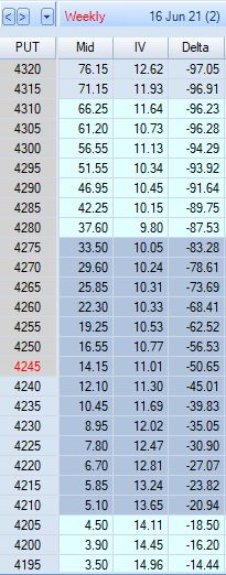
From the bottom, $3.50 to $3.90 is an increase in $0.40 per five point change in strike price. Moving up: $0.60, $0.60, $0.75, $0.85, $0.90, $1.15, $1.50, $1.65, and $2.05 brings us to the 4245 ATM strike. Per five point increase in strike price, the options usually increase much less than half that amount.

ITM premium differentials tell a different story. Going from ATM upward in 5-point increments, we see premium differences of: $2.40, $2.70, $3.05, $3.55, $3.75, $3.90, $4.10, $4.65, $4.70…

I collect closest to $1/point on the roll when DITM, which made me think whether I do the roll with few or many DTE, the essential element is to roll when DITM.

This analysis, however, misses the separate contribution of EV. EV is almost nonexistent near expiration but farther out, it can be seen as [log]normally distributed around the current price. Let’s revisit the option chain with time premium instead of delta displayed in the fourth column:

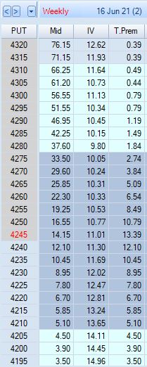
Again, premium differences from one strike to the next are much greater for ITM options than OTM. These differences approach $5, but T.Prem (EV) makes up the difference when less. The $13.39 EV for the ATM strike may be considered a “head start” for premium differences less than $5 as we walk the chain higher. I won’t secure point-for-point value for most rolls, but EV will make up for the shortage.

My current theory is that regardless of when, I want to be sure to roll while the option is ITM (or DITM) in order to avoid LIVOC. The option prices deceive by making higher-delta rolls seem more efficient since premium differentials approach $5. Either way, though, I will have realized point-for-point value for market movement up to my sold strike in addition to any EV the option had at the time I sold anywhere on the chain at expiration when all EV has evaporated. Remaining ITM allows further gains as the market moves higher.

I will continue next time.