Testing the Randomized OOS (Part 2)
Posted by Mark on January 30, 2019 at 06:35 | Last modified: June 15, 2020 06:36I described the Randomized OOS in intricate detail last time. Today I want to proceed with a method to validate Randomized OOS as a stress test.
I had some confusion in determining how to do this study. To validate the Noise Test, I preselected winning versus losing strategies as my independent variable. My dependent variables (DVs) were features the software developers suggested as [predictive] test metrics (DV #1 and DV #2 from Part 1). I ran statistical analyses on nominal data (winning or losing OOS performance, all above zero or not, Top or Mid) to identify significant relationships.
I thought the clearest way to do a similar validation of Randomized OOS would be to study a large sample size of strategies that score in various categories on DV #1 and DV #2. Statistical analysis could then be done to determine potential correlation with future performance (perhaps as defined by nominal profitability: yes or no).
This would be a more complicated study than my Noise Test validation. I would need to do subsequent testing one at a time, which would be very time consuming for 150+ strategies. I would also need to shorten the IS + OOS backtesting period (e.g. from 12 years to 8-9?) to preserve ample data for getting a reliable read on subsequent performance. I don’t believe 5-10 trades are sufficient for the latter.*
Because Randomized OOS provides similar data for IS/OOS periods, I thought an available shortcut might be to study IS and look for correlation to OOS. My first attempt involved selection of best and worst strategies and scoring the OOS graphs.
In contrast to the Noise Test validation study, two things must be understood here about “best” and “worst.” First, the software is obviously designed to build profitable strategies and it does so based on IS performance. Second, a corollary to this is that even those strategies at the bottom of the results list are still going to be winners (see fifth paragraph here to see that the worst Noise Test validation strategies were OOS losers). I still thought the absolute performance difference from top to bottom would be large enough to see significant difference in the metrics.
I will continue next time.
* — I could also vary the time periods to get a larger sample size. For example, I can backtest from
2007-2016 and analyze 2017-2019 for performance. I can also backtest from 2010-2019 and
analyze 2007-2009 for performance. The only stipulation is that the backtesting period be
continuous because I cannot enter a split time interval into the software. If I shorten the
backtesting period even further, then I would have more permutations available within the 12
years of total data as rolling periods become available.
Testing the Randomized OOS (Part 1)
Posted by Mark on January 27, 2019 at 06:28 | Last modified: June 14, 2020 08:00I previously blogged about validating the Noise Test on my current trading system development platform. Another such stress test is called Randomized OOS (out of sample) and today I begin discussion of a study to validate that.
While many logical ideas in Finance are marketable, I have found most to be unactionable. The process of determining whether a test has predictive value or whether a trading strategy is viable is what I call validation. If I cannot validate Randomized OOS then I don’t want to waste my time using it as part of my screening process.
The software developers have taught us a bit about the Randomized OOS in a training video. Here’s what they have to say:
- Perhaps our strategy passed the OOS portion because the OOS market environment was favorable for our strategy.
- This test randomly chunks together data until the total amount reaches the specified percentage designated for OOS.
- The strategy is then retested on the new in-sample (IS) and OOS periods to generate a simulated equity curve.
- The previous step is repeated 1,000 times.
- Note where the original backtested equity curve is positioned within the distribution [my dependent variable (DV) #1].
- Watch for cases where all OOS results are profitable [my DV #2]; this should foster more confidence that the original OOS period is truly profitable because no matter how the periods are scrambled, OOS performance will likely be positive.
I want to further explain the second bullet point. Suppose I want 40% of the data to be reserved for OOS testing. The 40% can come at the beginning or at the end. The 40% can be in the middle. I can have 20% at the beginning and 20% at the end. I can space out 10% four times intermittently throughout. I can theoretically permute the data an infinite number of times to come up with different sequences, which is how I get distributions of simulated IS and OOS equity curves.
Here are a couple examples from the software developers with the left and right graphs being IS and OOS, respectively, and the bold, blue line as the original backtested equity curve:
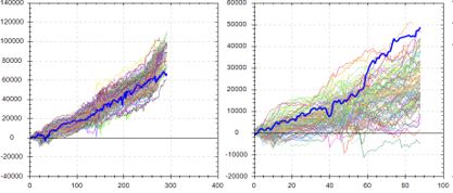
This suggests the backtested OOS performance is about as good as it could possibly be. Were the data ordered any other way, performance of the strategy would likely be worse: an ominous implication.
Contrast to this example:
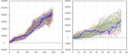
Here, backtested OOS performance falls in the middle (rather than top) of the simulated distribution. This suggests backtested OOS performance is “fair” because ~50% of the data permutations have it better while ~50% have it worse. This is considered more repeatable or robust. In the previous example, ~100% of the data permutations gave rise to worse performance.
The third possibility locates the original equity curve near the bottom of the simulated distribution.* This would occur in a case where the original OOS period is extremely unfavorable for the strategy—perhaps due to improbable bad luck. Discarding the strategy for performance reasons alone may not be the best choice in this instance.
I will continue next time.
* — I am less likely to see this because the first thing I typically do is look at
IS + OOS equity curves and readily discard those that don’t look good.
Automated Backtester Research Plan (Part 9)
Posted by Mark on January 24, 2019 at 06:27 | Last modified: November 23, 2018 09:40With digressions on position sizing for spreads and deceptive butterfly trading plans complete, I will now resume with the automated backtester research plan.
We can study [iron, perhaps, for better execution] butterfly trades entered daily from 10-90 days to expiration (DTE). We can center the trade 0% (ATM) to 5% OTM (bullish or bearish) by increments of 1% [perhaps using caution to stick to the most liquid (10- or 25-point) strikes especially when open interest is low*]. We can vary wing width from 1-5% of the underlying price by increments of 1%. We can vary contract size to keep notional risk as consistent as possible (given granularity constraints of the most liquid strikes).
An alternative approach to wing selection would be to buy longs at particular delta values (e.g. 2-4 potential delta values for each such as 16-delta put and 25-delta call). This could be especially useful to backtest asymmetrical structures, which are a combination of symmetrical butterflies and vertical spreads (as mentioned in the second-to-last paragraph here).
With trades held to expiration, I’d like to track and plot maximum adverse (favorable) excursion for the winners (losers) along with final PnL and total number of trades to determine whether a logical stop-loss (profit target) may exist. We can also analyze differences between holding to expiration, managing winners at 5-25% profit by increments of 5%, or exiting at 1-3x profit target by increments of 0.25x. We can also study exiting at 7-28 (proportionally less on the upper end for short-term trades) DTE by increments of seven.
As an alternative not previously mentioned, we can use DIT as an exit criterion. This could be 20-40 days by increments of five. Longer-dated trades have greater profit (and loss) potential than shorter-dated trades given a fixed DIT, though. To keep things proportional, we could instead backtest exiting at 20-80% of the original DTE by increments of 15%.
Trade statistics to track include winning percentage, average (avg.) win, avg. loss, largest loss, largest win, profit factor, avg. trade (avg. PnL), PnL per day, standard deviation of winning trades, standard deviation of losing trades, avg. days in trade (DIT), avg. DIT for winning trades, and avg. DIT for losing trades. Reg T margin should be calculated and will remain constant throughout the trade. Initial PMR should be calculated along with the maximum value of the subsequent/initial PMR ratio.
We can later consider relatively simple adjustment criteria. I may spend some time later brainstorming some ideas on this, but I am most interested at this point in seeing raw statistics for the butterfly trades.
I will continue next time.
* This would be a liquidity filter coded into the backtester. A separate study to see how open interest for
different strikes varies across a range of DTE might also be useful.
Butterfly Skepticism (Part 4)
Posted by Mark on January 21, 2019 at 06:37 | Last modified: November 23, 2018 10:14Today I want to complete discussion of the protective put (PP) butterfly adjustment.
I might be able to come up with some workaround (as done in this second paragraph) for PP backtesting. I could look at EOD [OHLC] data and determine when the low was more than 1.6 SD below the previous day’s close. In this case, I could purchase the put at the close. This would bias the backtest against (not a bad thing) the adjustment in cases where the close was more than 1.6 SD below because the put would be more expensive.
Unfortunately, I am not sure this particular workaround would work. If the close is less than 1.6 SD below then the backtested PP would be less expensive than actual. Furthermore, if I waited until EOD then the NPD and corresponding PP(s) to purchase would be different. This would distort the study in an unknown direction. I could track error (difference) between -1.6 SD and closing market price. Positive and negative error might cancel out over time. If I had a large sample size then this might or might not be meaningful.
At best, this workaround seems like a questionable approximation of an adjustment strategy that is precisely defined.
Before dismissing the PP out of frustration, let’s step back for a moment and piece together some assumptions.
First, I believe the butterfly can be a trade with somewhat consistent profits and occasionally larger losses. Overall, I’m uncertain whether this has a positive or negative expectancy (hopefully to be determined as I begin to describe here).
Second, as butterflies are held longer, I believe profitability will be decreased. I have seen some anecdotal (methodology incompletely defined) research to suggest butterflies are more profitable when avoiding periods of greatest negative gamma.
Third, I have seen anecdotal (methodology incompletely defined) research to suggest PPs as unprofitable whether:
- purchased in high or low IV
- purchased at specified deltas
- purchased for specified amounts
- held to expiration, managed at specified profit targets, or managed at 50% loss
Fourth, this adjustment will require any butterfly to be held longer on average. The additional time will be needed to recoup the PP loss. The result will be, as described per second assumption above, decreased average profitability.
In my mind, combining the first and fourth assumptions does not bode well.
The big unknown involves the magnitude of the largest losses and in what percentage of trades those largest losses occur.
Interestingly, the trader who explained this to me said PP will lose money in most cases. What it can prevent is a massive windfall loss. Being forthright [about the obvious?] may give the teacher more credibility. Without backtesting, though, I think it leaves us with more than reasonable doubt over whether this approach tends toward profit or loss.
Categories: Option Trading | Comments (0) | PermalinkButterfly Skepticism (Part 3)
Posted by Mark on January 17, 2019 at 07:13 | Last modified: November 23, 2018 09:58On my mind this morning is skepticism regarding the protective put (PP).
I have seen the PP lauded by many traders as a lifesaving arrow to have in the quiver.
One trader described this to me with regard to a butterfly trading plan. Part of the plan provides for the following adjustment:
- If NPD is at least 10 with market at least -1.6 SD intraday then record NPD.
- Buy PP(s) to cut NPD by 75%.
- On a subsequent big move, if NPD again reaches value recorded in Step 1 then repeat Step 2.
- If market reverses to the high of purchase day, then close PP(s) from Step 2.
Upon further questioning, I got some additional information. He learned it from a guy who claims to have “mentored” many traders. The mentor (teacher) claims to have seen many lose significant money in big moves and therefore recommends this to avoid windfall losses. The teacher has shown numerous historical examples where this adjustment would keep people in the trade (not stopped out at maximum loss) and often wind up profitable. Further prodding revealed uncertainty over whether these “numerous” examples amount to more than a handful of instances. Of the several times the adjustment has been presented, he acknowledged the possibility that many could have been repetition of the same [handful of] instance[s]. He is uncertain whether anyone has presented big losing trades more than once.
Much of this casts doubt over the sample size behind this adjustment. We certainly wouldn’t want to fall prey to that described in this this second-to-last paragraph.
As described in this third paragraph, the PP is simply an overlay added later in the trade. This strategy also has its own catchy name and is marketed. In order to backtest, we could study the profitability of long puts purchased on days the market is down at least 1.6 SD (also explore the surrounding parameter space as discussed in the fourth complete paragraph here).
From a backtesting perspective, intraday is a huge wrinkle. Technically, I’d need intraday data to identify exactly when the market was down 1.6 SD in order to purchase the PP at the correct time. As mentioned in the second-to-last paragraph here, this is arguably another reason why certain trading plans cannot be backtested: data not available.
I will continue next time.
Categories: Option Trading | Comments (0) | PermalinkConstant Position Sizing of Spreads Revisited (Part 4)
Posted by Mark on January 8, 2019 at 07:23 | Last modified: November 8, 2018 10:54Today I will conclude this blog digression by deciding how to define constant position size, which I believe is important for a homogenous backtest.
The leading candidates—all mentioned in Part 3—are notional risk, leverage ratio, and contract size.
Possible means to achieve—both mentioned in Part 2—are fixed credit and fixed delta.
I thought it might be the case that fixed delta results in a fixed leverage ratio. I suggested this in the last paragraph of Part 1 where I asked whether fixed delta would lead to a constant SWUP percentage. For naked puts under Reg T margining, gross requirement is notional risk. For spreads under Reg T margining, notional risk is spread width x # contracts and while notional risk may be fixed, the SWUP percentage varies.
Speaking of, we also have Reg T versus portfolio margining (PM) to complicate things. Both focus on a fixed percentage down (e.g. -100% for Reg T vs. -12% for PM) on the underlying. However, PnL at -12% can vary significantly with underlying price movement. PnL for spreads at -100% will not change as the underlying moves around because the long strike—at which point the expiration risk curve goes horizontal to the downside—is so far above.
Implied volatility (IV) also needs to be teased out since it will affect some of these parameters but not others. Given fixed strike price, IV is directly (inversely) proportional to delta (relative moneyness). For naked puts assuming constant contracts and fixed delta, IV is inversely proportional to notional risk and to leverage ratio. IV does not relate to leverage ratio for spreads, which is net liquidation value (NLV) divided by notional risk as defined two paragraphs above in the last sentence.
After spending extensive time immersed in all this wildly theoretical stuff, I seem to keep coming back to notional risk, leverage ratio, and fixed delta. The first two vary with NLV* and with # contracts due to proportional slope of the risk graph. Number of contracts can vary to keep notional risk relatively constant as strike price changes but this applies more to naked puts and less to spreads where spread width is of equal importance.
I want to say that for naked puts, the answer is fixed notional risk (strike price x # contracts), but we also need to keep delta fixed to maintain moneyness. With fixed credit, changing the latter would affect slope and leverage ratio. This is how I described the research plan originally and we will see whether an optimal delta exists or whether results are similar across the range. In the midst of all this mental wheel spinning, I seem to have gotten this right for naked puts without realizing it.
I guess I have also lost sight of the fact that this post is not even supposed to be about nakeds (see title)!
Getting back to constant position sizing of spreads, I think we can focus on notional risk and moneyness but we should also factor in SWUP. As the underlying price increases (decreases), spread width can increase (decrease) and we will normalize notional risk by varying contract size. Short strikes at fixed delta will be implemented and compared across a delta range.
Which is what I had settled on before (for spreads)…
[To reaffirm] Which is what I had settled on before (for naked puts)…
As I unleash a gigantic SIGH, I question whether any of this extensive deliberation was ever necessary in the first place?
I think at some level, this mental wheel spinning is what I missed as a pharmacist. The complexity fires my intellectual juices and is great enough to require peer review/collaboration to sort through. Once that is done, selling the strategy is an entirely separate domain suited to different talents, perhaps.
I left a job of the people (co-workers/customers) for a job that begs for people, which I have really yet to find. Oh the irony!
* By association, this is why I stressed magnitude of drawdown as a % of initial account value (NLV) in previous posts.
Constant Position Sizing of Spreads Revisited (Part 3)
Posted by Mark on January 3, 2019 at 06:45 | Last modified: November 7, 2018 05:17Happy New Year, everyone!
The current blog mini-series has been a tangent from the automated backtester research plan. Today I will discuss whether fixed notional risk—with regard to naked puts and spreads—is even important.
This issue is significant because it seems like fixed notional risk is the “last man standing” since I initially mentioned it in Part 1. I have reassessed the importance of so many concepts and parameters in this research plan. The fact that they get misunderstood and reinterpreted is testament to how theoretical and highly complex they are. Especially from the perspective of avoiding confirmation bias, I believe this is all debate that must be had, and a main reason why system development is best done in groups as a means to check each other.
The reason fixed notional risk may not matter is because leverage ratio can vary. I also mentioned this in the third-to-last paragraph here. Leverage ratio is notional risk divided by portfolio margin requirement (PMR). Keeping PMR under net liquidation value and meeting the concentration criterion are essential to satisfy the brokerage. Leverage ratio can be lowered by selling the same total premium NTM. This will affect the expiration curve by decreasing margin of safety as it lifts T+x lines. Analyzing this, somehow, might be worth doing if backtesting over a delta range does not provide sufficient comparison.
Whether “homogeneous backtest” should mean constant leverage ratio throughout is another highly theoretical question that is subject to debate. Keeping allocation constant, which I aim to do in the serial, non-overlapping backtests, is one thing, but leverage can vary in the face of fixed allocation. I discussed this here in the final four paragraphs. In that example, buying the long option for cheap halves Reg T risk but dramatically increases the chance of blowing up (complete loss) since the market only needs to drop to 500 rather than zero. While the chance of a drop even to 500 is infinitesimal, theoretically it could happen and on a percent of percentage basis, the chance of that happening is much greater than a drop to zero.
Portfolio margin (PM) provides leverage because the requirement is capped at T+0 loss seen 12% down on the underlying. In the previous example, 500 represents a 50% drop. Even under PM, though, leverage ratio can vary because of what I said in second-to-last sentence of paragraph #4 (above).
When talking just about naked puts, much of this question about leverage seems to relate to how far down the expiration curve extends at a market drop of 12%, 25%, or 100%. This brings contract size back into the picture because contract size is proportional to downside slope of that curve.
With verticals, though, number of contracts is less meaningful because width of the spread is also important. The downside slope will be proportional to number of contracts. The max potential loss of the vertical depends not only on the downside slope, but for how long that slope persists because the graph only slopes down between the short and long strikes.
Either way, you can see how number of contracts gets brought back into the discussion and could, itself, be mistaken as being sufficient for “constant position size.”
I certainly was not wrong with my prediction from the second paragraph of Part 1.
Categories: Option Trading | Comments (0) | Permalink