Call Me Crazy (Part 6)

I left off talking about RAR by PMDD. As impressive as this is in favor of the long call (LC) over stock shares, let’s consider the possibility that exposure isn’t everything.

Although a big difference exists between what is probable and what is possible, suitability standards for wealth management are based on the latter. The S&P 500 has never gone to zero* and I can hardly imagine a scenario where this happens in a sustainable society (I have seen fearmongers, omnipresent in the financial media, include Purge-like dystopias as part of their portrayal). Nevertheless, the possibility exists and risk models must respect it. We would otherwise be left to debate reasonable levels for maximum loss. Opinions on this differ and should we be wrong [likely, since “your worst drawdown is always ahead of you” (see third-to-last paragraph here)], the result could be tantamount to a true financial apocalypse.

[Deleveraged] Investing with insurance means we survive the worst. I’ve been in the trading trenches for the last 12+ years. Most of the time, things go smoothly. When markets get rocky, fear and stress mount fast. To have the confidence my portfolio will remain [healthy] even in the face of a total stock market collapse represents an enormous sense of security. Most substantial investors would feel the same way.

Backtesting the LC through the Great Recession appears quite encouraging.

Can we imagine a case where the strategy falters?

Consider how the LC fares in down markets. On the upside, the LC faces a performance drag in terms of upfront cost. An ATM (slightly OTM, actually) LC will expire worthless if the market does not go up. In the backtest, I purchased LEAPS two years to expiration and rolled after one. The market is marginally higher in two of the 14+ backtested years and only down in three. Is it true that overall, the LC fares better because most down years are small and/or because the LC retains most of its premium being closed with a full year left until expiration?

The second and fourth columns show % ROI for SPX share and LC accounts, respectively. The third column shows % ROI for the LC itself. Here are some observations:

• LC is battered and bruised in 2008 despite performing much better than the shares.
• LC underperformance during other four years averages 2.99% (not insignificant).
• LC average cost across all 15 periods (last being a partial year) is 16.10% (of account value).
• LC loses substantial value over first year in trade although hit to the entire account is less.

That final point has a lot to do with leverage. I have been enchanted by the limited exposure—how much firepowder remains dry—when investing with LCs. For a $100,000 account, every year offers the tempting opportunity to purchase up to 4 – 5 contracts. The last column increases proportionally to number of contracts, though. This is an ever-present threat.

I will continue next time.

* — SPX pulled back 57% from its all-time 2007 high by March 2009: the worst bear market
       many of us have ever experienced, but a far cry from total 100% loss.

Call Me Crazy (Part 4)

I’ve been digging into results from my backtest on the long call versus underlying stock shares. Last time I took a deep dive into the numbers behind RAR by MDD. Today I want to move forward.

MDD is based on a single occurrence, which is one thing I do not love about the risk metric. As discussed here, large sample sizes lower the possibility of fluke occurrence. This is difficult when starting with a set consisting of only one data point per year even enhancing with 24 points of additional context. Alternatives to MDD include top three DD’s (referenced in the fifth paragraph here), average of the top three DD’s, or distribution of DD’s.

RAR by standard deviation (SD) sidesteps the single-occurrence issue by looking at overall variability. For the enhanced data set, this is 9.53 for the long call vs. 5.57 for SPX shares. This is a 1.7-fold difference compared to 1.1x (7.48 versus 6.70) in favor of the long call in the original data set. This feels right* because the enhanced data set includes additional downside volatility and was precisely the motivation for my last post.

Looking at the equity graphs in Part 3, the enhanced data set exhibits additional curve crosses. March 2020 is the real eye-opener because a substantial lead accumulated by the SPX account for over a decade evaporates in one fell swoop before completely recovering within six months. What a ride, though: adrenaline junkies rejoice! This is the opposite of what seniors or anyone with retirement in their sights want to see.

SPX hits an all-time closing high (ATH) of 1565.15 on Oct 9, 2007. I’m tempted to include this in the enhanced data set to see how it would affect the numbers. ATH is a 10.49% increase from Jan 2007 where the long call is up 8.78%. I’m guessing inclusion would mitigate the difference between original and enhanced data sets for RAR by MDD, accentuate the difference for RAR by SD, and add a couple more crosses to the equity graph.

Whether the ATH should be included is debatable. I aim to understate backtesting differences to strengthen my beyond-a-reasonable-doubt (see last paragraph here) search for viable strategies going forward. The main reason not to include is that upside volatility will not result in loss. Main reasons to include are because upside volatility is very real and because upside volatility can result in psychological loss if DD’s are calculated from a highwater mark (potential topic for future blog post).

I will continue next time.

* — What doesn’t feel so right is the impressive result that long call SD decreases from 0.141 to 0.112
       between original and enhanced data sets where SPX-share SD increases from 0.160 to 0.191.

Mathematical Excursion

I left off by explaining the difference between MAR by MDD as more extreme for the original data set than for the enhanced data set. Since this seemed counterintuitive to me, let’s take some time to explain it.

I expected long call MAR by MDD to shine even brighter compared to shares given the enhanced data set. After all:

• I used the same formula for both: (100 * Geo. Mean) / MDD %.
• Between the start of 2009 and the market low on 3/9/2009 (additional enhanced data point), the long call account dropped from $79,956 to $67,309: -16.8%.
• The SPX account dropped an even greater percentage from $65,777 to $47,757: -27.4%.

What actually matters is not whether the SPX account dropped more during the additional 66 days but rather how the drop over the additional 66 days compares to the original Jan 2008 – Jan 2009 decline. For a proportional drop in both the long call and shares, I would expect the ratio of the enhanced RAR by MDD to be the same. With 1.0 reflecting proportionality, the ratio of MDD % for long call is 0.56 for the original data set and 0.62 for the enhanced thereby suggesting the drop is closer to proportionate through 3/9/09 than it is through Jan 2009. Put another way, the more proportionate additional 66 days dilutes RAR by MDD for both the long call and underlying shares.

A table may help:

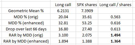
The numbers in bold are what puzzled me. The first and third numbers in the same column explain why. The ratio between MDD % is closer to 1.0 in the last 66 days, which evens out the overall comparison if only by a small amount.

Coincidentally, the ratio of the drop over those last 66 days (third number, last column) is very close to the ratio of MDD % for the enhanced data set. This got me thinking why these two numbers might be the same. They are not the same, though: 0.616 vs. 0.613. Pure coincidence.

When comparing RAR between groups, I make sure to calculate RAR in an identical manner. The idea is to divide return by some measure of risk because greater (lesser) risk should decrease (increase) RAR. I will sometimes multiply by a constant (100 in this case) to make the numbers easier to interpret. The constant doesn’t matter as long as I apply the same to both.

For these reasons, my RAR is not necessarily comparable to anyone else’s.

In and of itself, the term “risk-adjusted return” is non-specific. Different metrics for risk include alpha, beta, R-squared, and standard deviation (SD). The Sharpe ratio is a RAR metric that uses SD as its risk measure. The Treynor ratio is a RAR metric that uses beta as its risk measure.

I worried this excursion might take us out to the weeds. Indeed it has! I come back to reality (hopefully) next time.

Call Me Crazy (Part 3)

Today I want to contrast backtesting results presented in my last post between the long call and underlying shares.

While mulling over the results, I questioned whether I was doing a valid apples-to-apples comparison with regard to position sizing. Initial account value was $100,000 for each yet with SPX at 1416 on 1/3/2007, the notional value of one 1425 call is not $100,000 but rather [ ( underlying price – points OTM) * 100 ] $140,700.

This apparent discrepancy is much ado about nothing. Changes in underlying account value are proportional to changes in the underlying itself, which is what I used to calculate max drawdown (MDD). MDD may be calculated as a percentage, thereby normalizing for any scale difference. In reality, one long call may control more or less stock than the arbitrary $100,000 initial account value and is not germane to this discussion.

With that resolved, I now feel comfortable to show this:

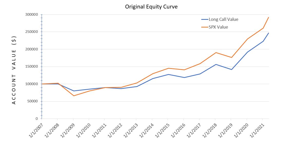
The greater stability of the long call (blue line) is seen in terms of a higher low and subsequent lower high. Aside from that, I think the table presented last time did more to illuminate differences.

What we really don’t see, which I continue to contemplate as a potential game changer, is the peace of mind coincident with a blue line that cannot lose any more in one year than it did in 2008. I will talk more about this later.

Speaking of psychology, both curves are deceptively smooth because they only contain one data point per year. The market moves around much more than this. While sharp selloffs can impart great fear among investors, owning a long call during a 2008-like selloff may put me near a loss level beyond which I can lose no more. I am therefore freed of the temptation to exit, which for shares often locks in catastrophic losses at the worst time (see last paragraph here). By holding on at market-crash lows, the only way for the call investor to go is up.

To get a better sense of actual volatility, I backtested 24 additional days between 2007 – 2020 where the underlying market hit near-term lows:*

The total return and starting/ending points are all the same in this enhanced graph. The additional data points highlight more of the downside volatility actually experienced.

Between the long call and long shares, MAR by MDD differs less in the enhanced data set than it does in the original: 3.27:1.99 (enhanced) versus 5.30:3.02 (original).

Why is this?

Next time, I will continue with a brief excursion into the weeds.

* — The actual MDD for all 5,244 days is not captured because I did not backtest any near-term highs.

Call Me Crazy (Part 2)

Last time, I presented a long call backtesting procedure. Today let’s get into some results.

I used OptionNet Explorer (ONE) to help me with the work. ONE is an excellent piece of software. At some point, I will do a complete review of ONE and compare it with OptionVue.

This backtest goes from Jan 3, 2007, through May 13, 2021:

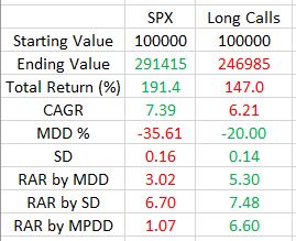
SPX outperformed in terms of total return and compound annualized growth rate (CAGR): annualized return geometric mean.

All of the volatility metrics are in favor of the long call. Maximum drawdown (MDD) is 43% lower for the long call. While it’s bad practice to take a percentage of a percentage (see fourth paragraph here), risk-adjusted return (RAR) by MDD is much better for long call. As MDD is based on one occurrence (2008, in this case), I also calculated RAR by standard deviation to get a broader overview. This still favors the long call albeit only slightly.

Maximum potential DD (MPDD) is how much I can possibly lose were the market to go to zero. For a long call, this is limited as shown in the risk graph here. Until expiration, all I can lose is the amount I paid for the call. With shares, I can lose 100%.

Let’s illustrate with an example. On Jan 3, 2007, SPX traded at 1416.6 and the Dec 2009 1425 call went for $155.20. For the right to buy 100 shares of stock, then, I paid $15,520. The value of 100 shares of stock was $141,660.* Were the stock market to crash and go to zero, I would lose $15,520 owning a long call versus $141,660 owning the shares.

Not a perfect analogy (by any stretch), but a long call is like “paying rent” to participate in stock returns where the most I can lose is the rent itself. If the house is destroyed, then I do not lose the value of the house. If the stock market goes to zero, then I do not lose the total value of the stock. With regard to ultimate risk, such deleveraging may be a game changer. This is why the 60/40 stock-bonds portfolio has long been championed as a diversified portfolio by the financial industry.

I think deleveraging should somehow be factored into RAR because deleveraging lets people sleep well at night (I discussed importance of RAR in the fifth paragraph here). Here, RAR by MPDD is six times better for the long call than underlying stock.

More caveats to be considered next time.

* — SPX cannot be purchased directly. The SPY ETF would suffice, and since its price is 1/10
       that of the index, 100 * 10 = 1000 shares could be used as a proxy.

Call Me Crazy (Part 1)

In these two posts, I started to introduce components I am considering for a new portfolio investment approach. In this post, I will present a long call backtesting approach.

In my opinion, the long call risk graph has one very attractive potential feature: built-in insurance. I included the risk graph in Part 1 (linked above). Notice the horizontal line that extends leftward to zero. That represents a range of prices for the underlying where PnL at expiration does not change. Although I won’t discuss it any further here, this feature makes the long call a prime candidate for “cash replacement.”

When position sized properly, the long call acts like insurance because the premium I pay up front is the most I can lose until expiration. What I need to thoroughly understand is annual cost as a percentage of the underlying. The cost drags down total return, which is bad. The good thing is that I should feel completely safe in case the market goes down. Good, good, good—this is my main reason for being here today.

To gain more understanding of long calls, I conducted a backtest as follows:

• On first trading day of year, BTO the first OTM call with expiration in December two years hence.
• If underlying falls within a couple points of a strike price, then buy ATM option instead.
• Include $1.00 per contract for commission.
• Factor in [aggressive] slippage by selecting price 20% of the way between natural and mark.
• On first trading day of next year, STC the long call.
• BTO a new long call as described above.

Data columns included:

• Date and DTE
• Underlying price strike
• Round trip commission
• Mark and actual prices for open and close
• Current cost
• Maximum ($) potential loss
• Maximum (%) potential drawdown (MPDD) for account and underlying
• Account and underlying annual ROI

Initial metrics to compute included:

• Cumulative return
• Geometric mean
• Annualized return
• Standard deviation (SD)
• Maximum drawdown (MDD)
• Risk-adjusted return by SD, by MDD, and by MPDD

I will present results next time.

Backtesting Issues in ONE (Part 3)

Last time, I delved deeper into some crazy-looking data I have seen in OptionNet Explorer (ONE) and why it makes little sense. Today I will finish up.

One thing I wonder is whether part of this has to do with inaccurate quotes approaching the close. For example, on 5/7/21 at 3:55 PM EDT, SPX was ~4231. With 7 DTE, the 4275 put (OI = 22) is listed at 46.60 / 54.40. At $7.80, that is wide enough to drive the proverbial truck through! Another trader said:

     > I don’t know what BD you use, but the SPX bid/ask spread on an option
     > 7 DTE with Fidelity is seldom greater than $2—usually between $1 – $2.

This was puzzling because I see wide spreads like this often in ONE. I backed up to 3:30 PM and with SPX ~4236 (OI still 22), the same 4275 put shows 48.40 / 49.00. What an enormous difference! I would trade the latter all day long. With the former, I’d be concerned that slippage might completely offset my edge.

I have heard many times that bid/ask spreads frequently widen after the close rendering EOD quotes unreliable. Could this apply to 3:55 PM? I would actually think this would be smack dab in the busiest, most liquid part of the trading session when bid/ask spreads are narrowest and quotes are most accurate.

EOD liquidity may also pertain to quote freshness. I’m not talking about Sara Lee bread here, but rather how recently the option last traded. An option that has not traded for days (if ever) will likely show a stale quote. Quotes from liquid times of the day are less likely to be stale because higher-volume trading is taking place, but this is a probability: not a guarantee. In the example above, constant OI (22) suggests the option may not have been traded [between 3:30 and 3:55 PM], which then begs my question why the spread would be jacked wide open 25 minutes hence.

I will not backtest with quotes that violate strike arbitrage. I simply cannot believe I would actually see those numbers in real-time despite ONE Customer Support claiming this to be the case [and if I did, then I should immediately arb it regardless of what my current strategy calls for]. Even if I could salvage the exorbitant bid/ask spreads seen on ONE by moving the whole quote up or down to get a valid option chain, it would require spreadsheet manipulation and be a hassle to do.

Open Interest (OI) may be germane to this discussion. OI is 22 in the example given above. This is relatively high compared to what I see on the DITM puts in 2007-2009, which often have slim to no OI. This makes me wonder about a couple things. First, with such low OI am I seeing stale quotes that would change markedly were I to actually place an order? Second, is low OI a real cause of larger slippage? Given ONE data, round-trip slippage for ~5% ITM SPX naked puts in 2007 averages just over $1.30. With slippage factored in, maybe the sticky extrinsic no longer violates strike arbitrage.*

One final consideration regards a methodological tweak I applied in backtesting before Weeklys became available. These particular trade guidelines called for selling 1% ITM with 7 DTE. Before Weeklys, I sold 4-5% ITM on options 4-5 weeks to expiration. The former may be much more liquid than the latter for two reasons. First, near-dated options are usually more liquid than far-dated. Second, expected move is not directly proportional as applied here but rather proportional to the square root of time. Relatively speaking, I was therefore using options even deeper ITM.

I may not be able to backtest with these quirky option prices at least until I have more experience trading similar options to know what usual slippage and bid/ask spreads are like. For now, I should trade small and consider starting my backtest later in the data set when quotes are more reliable. Once I have gained a familiarity with these particular options, I can apply what I know to correct any seemingly distorted quotes from ONE.

* — This would not be the case if bid/ask spread is also similar across a range of strikes.

Backtesting Issues in ONE (Part 2)

Last time, I presented some screenshots detailing quirky things I have been seeing in OptionNet Explorer (ONE) pertaining to data. Today I will continue the discussion.

My initial thought was that I should not be seeing zero extrinsic value across a range of strikes with significant time to expiration. If the benefits of early put exercise (i.e. earning risk-free rate on the proceeds) outweighs the extrinsic value, then the put should be exercised early. Since extrinsic value is surrendered upon exercise, put buyers can exercise ITM options without penalty once extrinsic value is gone. They can then implement the proceeds elsewhere.

If what I am seeing in ONE were accurate, then early exercise should be common. Based on my experience and what I hear from others, it is not.

Wait! I now realize I made a major oversight here. Looking back at the screenshots, do you see it?*

The more general case of seeing constant (“sticky”) nonzero extrinsic value across a wide range of strikes also seems wrong.

I e-mailed ONE Support on this issue and got some meaningful information. I strongly praise DJ who has been very helpful and usually prompt with his response time. He writes:

     > The data isn’t corrupt but you will notice wider spreads on some
     > instruments, particularly SPX when using EOD quotes. These were
     > the exact quotes provided by CBOE so they are accurate and exactly
     > what you would have seen in the market at that point in time when
     > viewed at the EOD…
     >
     > I note what you refer to as the “sticky” nature of some of the
     > quotes but again, they are correctly derived from the market data.
     > Our beta version shows both bid and ask prices (as well as mid
     > price), and you will notice up to $3 spreads on some strikes at
     > the EOD. This can inevitably impact the calculation of both IV and
     > extrinsic value, depending on where the mid price resides and
     > how the spread widens.

Provided we believe DJ, which I do, the data seen in ONE are accurate.

I remain troubled because these inconsistencies seem to violate option arbitrage. As an example with the underlying at 100, suppose the 105 and 110 puts are priced at $5 and $10, respectively: both having zero extrinsic value. I could then sell the credit spread for $5 and have a position that would at worst lose nothing (options expire ITM) and at best profit $5 (options expire worthless). This edge would be exploited repeatedly until it went away (selling causes extrinsic value to decrease while buying causes extrinsic value to increase).

A range of options having constant nonzero extrinsic value should similarly violate option arbitrage. With the underlying at 100, suppose the 105 and 110 puts are priced at $8 and $13, respectively: both having $3 extrinsic value. I could then sell the spread and have a max potential profit of $5 (options expire OTM) with a max potential loss of breakeven (options expire ITM). Again, this edge would be exploited repeatedly until it disappeared.

I question whether flawed numbers like this can be used to backtest, and I remain puzzled as to why I am seeing it.

I will continue next time.

* — SPX has cash-settled, European options that are not subject to early exercise.

Backtesting Issues in ONE (Part 1)

I recently subscribed to OptionNET Explorer (ONE). ONE is option analytics software that has been around for many years. I have started my ONE backtesting journey with ITM puts and have run into questions about data integrity.

I started backtesting in 2007. Look at the following screenshot:

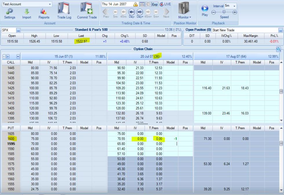
The underlying is at 1522.97. I highlighted the 1600 strike, which is roughly 1% ITM/week compounded geometrically. Zero extrinsic value (T.Prem column) is displayed. In fact, a range of strikes show zero extrinsic value down to the 1565 strike. With five weeks to expiration, this doesn’t feel right to me even being DITM.

Look at the OTM portion of the option chain:

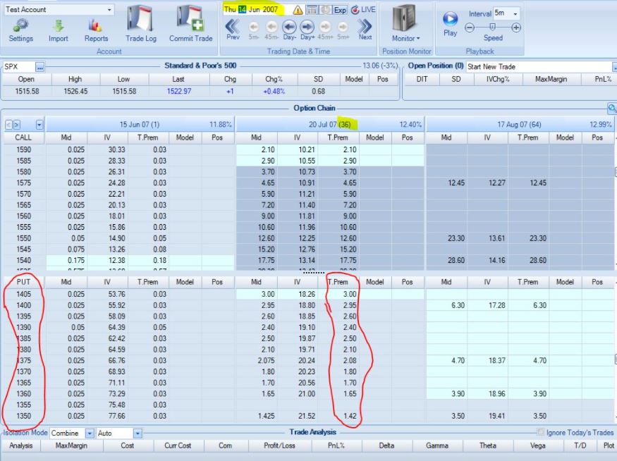
These puts have extrinsic value well into the third standard deviation. Vertical volatility skew would dictate OTM puts to have a higher implied volatility (more extrinsic value) than calls OTM by the same amount (referred to as moneyness). I believe this also pertains to ITM vs. OTM puts. Assuming this to be true (especially so if not), I still question what we’re seeing here. The option chain shows DOTM puts with extrinsic value well beyond the second standard deviation compared to ITM puts with zero extrinsic value less than a full standard deviation out.

The following screenshot feels about right to me:

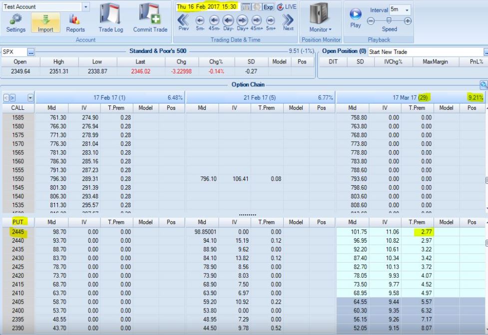
Extrinsic value should be greatest ATM and proportionally decline with moneyness. Whether the relationship is like an inverse V or a bell curve, what we see here seems much more reasonable. We shouldn’t see all zeroes.

I used to use OptionVue and I would sometimes have similar issues with their data. It didn’t seem to be every day, certainly, but before 2008-2009 or so, it was somewhat prevalent.

I will continue next time.

* — One standard deviation equals underlying price * implied volatility (decimal) * SQRT ( DTE / 365)