Trading System #1–SPY VIX (Part 10)

In http://www.optionfanatic.com/2012/10/25/trading-system-1-spy-vix-part-9, I presented a MAE graph that damaged any hopes for implementing a protective stop-loss.  Today I want to nail this down and make a decision.

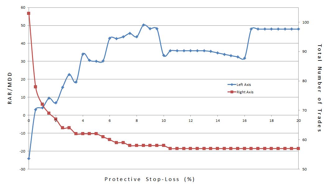
The MAE graph can only hint indirectly about an optimal stop-loss level.  A graph of the subjective function vs. different stop levels is more definitive.  As with other graphs of the subjective function, what I want to see is a high plateau region rather than spikes or trends.  Below, RAR/MDD is plotted vs. stop-loss where the latter is varied from 0% to 20% by 0.5% increments:

The blue line trending from low to high with a dip in the middle suggests that the system becomes more profitable as the stop-loss is relaxed from zero.  The graph clearly shows why tight stops are seldom recommended.  While the middle is a plateau region, the fact that it is a valley rather than a peak suggests it is less profitable than a wider stop.

The dip is explained by one trade that had a MAE of 16.45% with a final loss of 0.2%.  A stop level up to 16.45% would have caused this trade to exit at the stop level (locking in a loss up to 16.45%).  Once the stop level exceeded 16.45%, however, the trade was allowed to rebound and lose the modest 0.2%.

The red line, which indicates total number of trades, decreases as the stop-loss increases.  This is because the more often trades are stopped out, the more additional days are freed up for new trades to be opened.  Recall that this system only trades one open position at a time.

In conclusion, I do not feel any protective stop-loss should be used with this system at all.  I will discuss this more in the context of position sizing.

Trading System #1–SPY VIX (Part 9)

In http://www.optionfanatic.com/2012/10/20/trading-system-1-spy-vix-part-8, I settled on x = 5 to complete selection of the three parameter values for the SPY VIX trading system.  It’s not ready for prime time just yet.  Today I will begin exploration into Maximum Adverse Excursion (MAE).

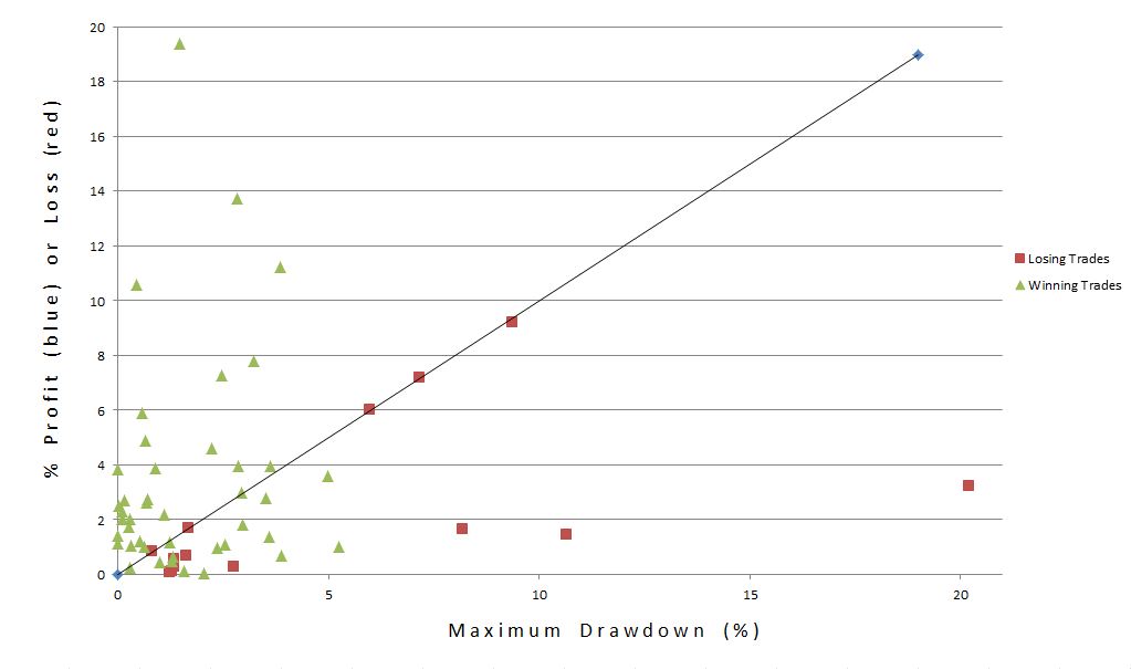
I described the process I am about to undertake in http://www.optionfanatic.com/2012/10/24/maximum-adverse-excursion.  Focusing specifically on x = 5, y = 25%, and z = 10, here is a scatter plot of P/L by maximum drawdown (MDD):

The triangles and squares are results of the 57 trades.  The higher the point, the greater the profit (green) or loss (red).  The farther to the right, the greater the MAE.  The [roughly] 45-degree line is called the loss diagonal, and it represents the maximum loss for red squares.  Losing trades can never be above the line because the most they can lose is the most they were ever losing (MDD).

A stop-loss would be represented by a vertical line on the graph.  Any losing trades to the right of the vertical line would then move to the intersection of the vertical line and the loss diagonal.  Any winning trades to the right of the vertical line would become red squares (losing trades) with height equal to the intersection between vertical line and loss diagonal.

What I want to see in order to implement a stop-loss is more of the former that lie above that intersection than below it and few of the latter.  Red squares to the right of the vertical line and above the intersection are trades that would be stopped out for a decreased loss (+1 for system).  Red squares to the right of the vertical line and below the intersection represent losing trades that would be stopped out before having a chance to recover (-1 for system).  Green triangles to the right of the vertical line represent winning trades that would be stopped out for losses before being able to recover into profit (-1 for system).

I don’t see a good place to draw the vertical line such that the +1’s substantially outweigh the -1’s.

Before dismissing a potential stop-loss for this system altogether, I will undertake one more analysis in the next post.

Trading System #1–SPY VIX (Part 8)

In http://www.optionfanatic.com/2012/10/19/trading-system-1-spy-vix-part-7, I finalized values for y (25%) and z (10).  Today, I want to make a final decision on x.

From statistical tables in http://www.optionfanatic.com/2012/10/16/trading-system-1-spy-vix-part-5 and http://www.optionfanatic.com/2012/10/19/trading-system-1-spy-vix-part-7, I have cherrypicked just the rows corresponding to y = 25% and z = 10:

As trade length increases, exposure will increase and RAR will consequently decrease (assuming all else remains equal).  This explains the trend lower in RAR/MDD as x increases from three to seven.  If I want the most concentrated returns then I should aim for the smallest x-value.

Stability of RAR/MDD across different values of z increases with trade length as evidenced by the trend lower in CV and Range (%) as x increases from three to seven.  This suggests I should aim for the largest x-value.

I am favoring x = 5, which will provide a decent RAR/MDD and stability therein.

Since RAR/MDD can obscure Net Profit, I want to add one additional column to the above table:

I am somewhat surprised to see Net Profit trail off when x > 5 because the longer the trade, the more opportunity for profit to accumulate.  It is possible that after five days mean reversion has occurred and no further edge is available.

The average number of trades for y = 25% is 55.7 (range = 34) across all values of z.  This is not a large sample size.  If it weren’t for the preponderance of positive numbers across all 150 systems and the trend toward more concentrated profit at higher y-values then I might abort this system altogether and look for something with more backtesting data.

Given all these considerations, I feel comfortable implementing SPY VIX with x = 5, y = 25%, and z = 10.

Trading System #1–SPY VIX (Part 7)

In http://www.optionfanatic.com/2012/10/17/trading-system-1-spy-vix-part-6, I determined that for x = 5, y = 25% produced the best backtesting results for z-values between 6-15 (see first paragraph of http://www.optionfanatic.com/2012/10/18/laziness-dissected for a refresher on the SPY VIX trading system).  I now want to see if this holds for x = 3 to 7.

Here is the graph and statistical analysis (lowest stability numbers in bold) for x = 3:

Here is the graph and statistical analysis (lowest stability numbers in bold) for x = 4:

Here is the graph and statistical analysis (lowest stability numbers in bold) for x = 6:

Here is the graph and statistical analysis (lowest stability numbers in bold) for x = 7:

Which value of y had the most stable curves as measured by lowest CV (SD / mean) and lowest Range (%) statistics?

No edge there…

The y = 25% curve prints the largest RAR/MDD for most values of z on all graphs.  Out of 50 total backtested systems, RAR/MDD was largest along the y = 25% curve 44 times (by random chance alone, one would expect 10).  Six times, y = 20% resulted in a larger RAR/MDD value.  These six cases occurred with z = 6 (once), z = 7 (three times), or z = 8 (twice).  Never did this occur for z-values of 9-15.

In conclusion, y = 25% is as consistent as any other y-value across all values of x and z.  Furthermore, y = 25% reliably scores highest on the subjective function RAR/MAD.  In looking at the five y = 25% curves, I would choose z = 10 as the center of the most consistent plateau region where the curve is least likely to fall off “precipitously” at neighboring z-values.  Even if the y = 25% curve does fall off, however, RAR/MAD is still very likely to be larger than curves of any other y-value and in all cases would still have generated respectable profit.

Trading System #1–SPY VIX (Part 6)

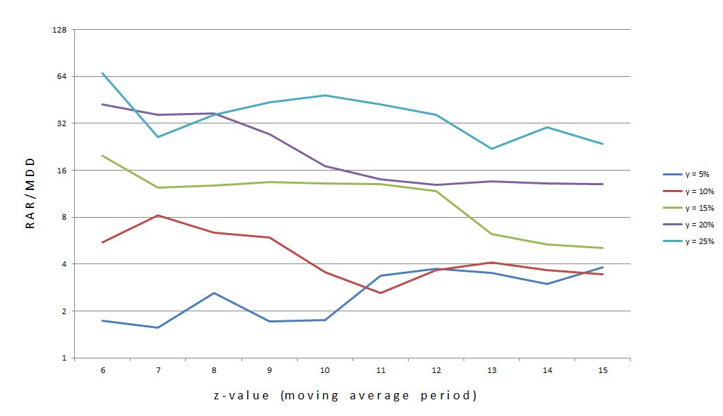
In http://www.optionfanatic.com/2012/10/16/trading-system-1-spy-vix-part-5/,  I took a close look at the subjective function RAR/MDD by % extended across moving average length (z).  I will continue that analysis today.

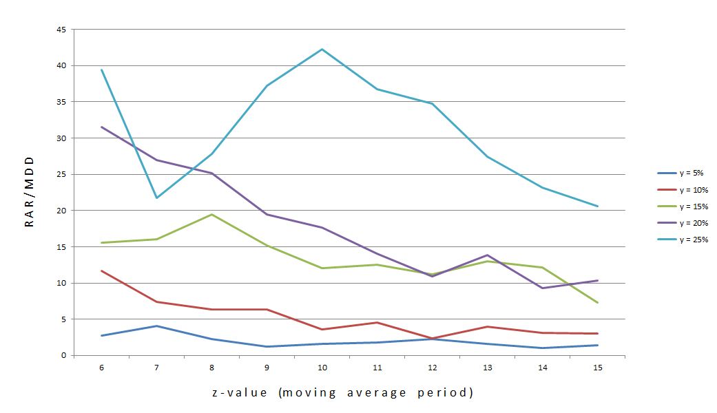
Let me begin by reposting Figure 1 from my last post:

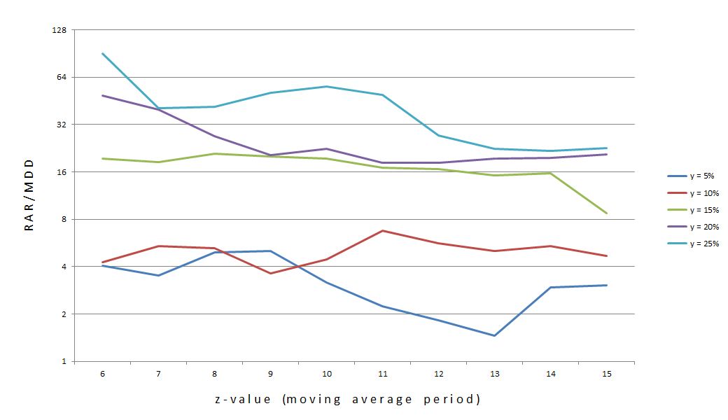
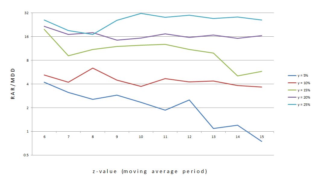
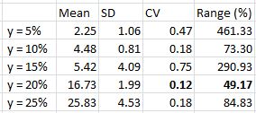
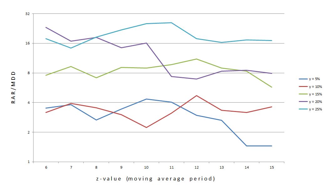
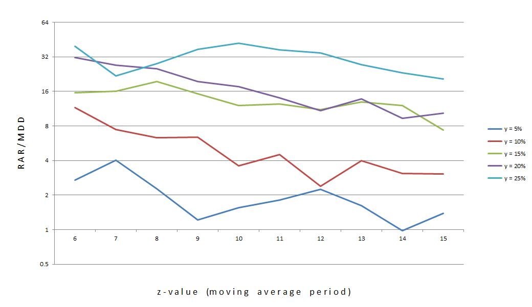
The statistics showed that y = 25% (top curve) is actually the flattest of the five.  Perhaps this graph is more convincing:

Do you see the difference?  The y-axis is logarithmic in the bottom one, which means any given length represents the same multiplier rather than addend.  Each tick on the y-axis multiplies the previous y-value by two rather than adding five.  This eliminates distortion caused by widely-ranging (in percentage terms) values.

In addition to choosing y = 25%, I will choose z = 10.  This is roughly the center of the middle, high plateau region of the curve.

Going back to Table 1 in http://www.optionfanatic.com/2012/10/16/trading-system-1-spy-vix-part-5/, another observation about these 25% extended systems is the low number of trades.  Indeed, a regression analysis shows that total number of trades and % extended are highly correlated (R-squared = 0.8921).  On average, these 25% extended systems traded 55 times over 20 years, which is just over 2.5 trades/year.

Despite trading infrequently, these 25% extended systems have been very profitable in the past.  Profit factor (PF) is positively correlated with % extended with an R-squared value of 0.7516.  The 25% extended systems have the highest average PF of all with an average of 3.13.

To recap, I have 2.5 trades/year x 5 days/trade = 11 days/year and 11 days/year x 1 year / 252 trading days = 4.4%.  If I can find 10 more systems that have a good basis for diversification then I can have be invested on roughly 50% of all trade-days (# trades x trading days invested) with good probability for concentrated profits (high PF).  A good basis for diversification includes mean-reverting and trend-following systems along with different (non-correlated) asset classes.

I’m not done developing this system, though.  In the next post, I will discuss the x-bar stop.

Trading System #1–SPY VIX (Part 5)

The subjective function is now in hand:  RAR/MDD.  I will now recreate the results presented in http://www.optionfanatic.com/2012/10/02/trading-system-1-spy-vix-part-3-2 and redo the consequent analysis.

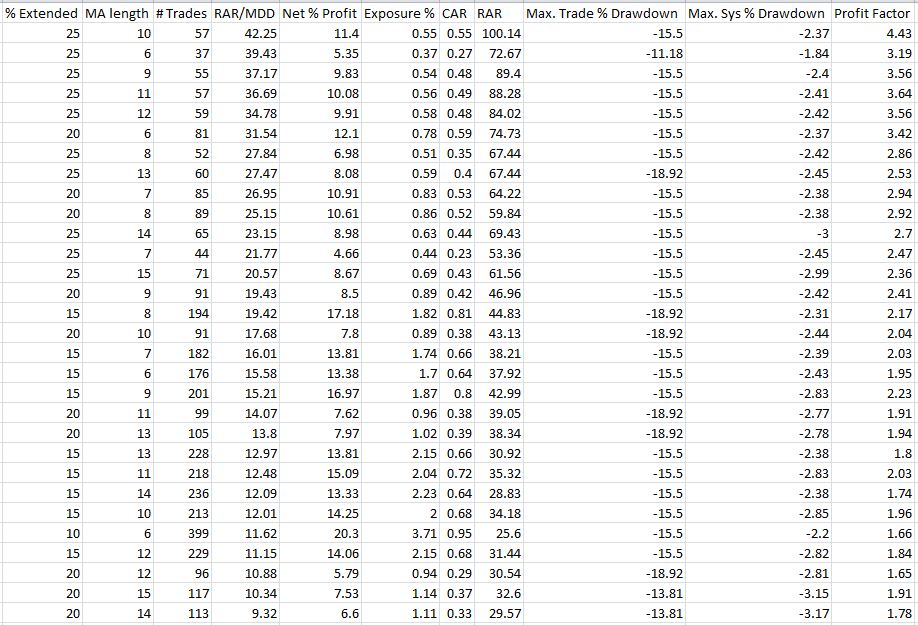
Here are the results for the top 30 parameter combinations as sorted by RAR/MDD:

Table 1

My first observation is that a cluster of 25% extended systems sit right at the top.  Indeed, running a linear regression analysis on all 50 systems shows that % extended and RAR/MDD are correlated with an R-squared value of 0.77 (R-squared > 0.80 is typically considered “strongly correlated”).

This makes logical sense as a mean-reversion trading system.  Mean-reversion systems are based on the idea that the farther the rubber band gets stretched, the more likely it is to snap back [to the mean].  The more extended VIX gets above or below the VIX moving average, the more likely SPX is to move higher or lower, respectively.  This was also seen [less clearly] in the graph of Net Profit % (http://www.optionfanatic.com/2012/10/03/trading-system-1-spy-vix-part-4/).

If I break down systems by z-value (moving average period), then the results look like this:

Figure 1

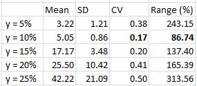
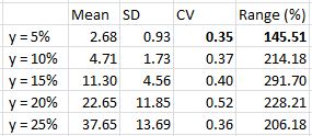
Keeping in mind that I want to see plateau regions rather than spike regions, the bottom curve (y = 5%) looks best.  The statistics do not bear this out, however:

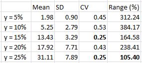
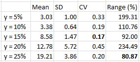
Table 2
Mean = average RAR/MDD
SD = Standard Deviation
CV = Coefficient of Variance (SD / mean)

The lower the SD, the flatter the curve.  Even more important is to interpret SD as a percentage of the mean since the means vary over 15-fold.  By that metric, y = 25% is the most consistent.

Indeed, y = 25% has a greater RAR/MDD over the entire range of z values.  Even the lowest RAR/MDD for y = 25% (at z = 7) is greater than the highest RAR/MDD for y = 15% (at z = 8).  Given these observations, y = 25% seems to be the best choice.

I will continue this analysis in the next post.

Trading System #1–SPY VIX (Part 4)

Today I will begin to analyze results of the SPY VIX trading system optimization study.  Please refer to Tables 2A and 2B from http://www.optionfanatic.com/2012/10/02/trading-system-1-spy-vix-part-3-2 for the backtest results.

My first observation is that each of the 50 parameter combinations leads to a profitable system!  Net profit % ranges from 4.66% to 20.30%.  Remember that the issue we’re ultimately trying to address is how probable it is that the system we are backtesting will generate profit going forward.  All parameter combinations backtesting profitably makes me more confident that the chosen system will be profitable in live trading than if all parameter combinations did not backtest profitably.

While this conclusion may seem obvious, it does head off the tendency to infer more from the observation than is actually presented.  Beginning (and seasoned!) traders are all-too-often eager to enter the market with any half-decent excuse for a [potentially] winning system, open their bags, and let the money fall in.  This is the allure/mirage of Wall Street (otherwise known in human nature terms as “greed”).  The harsh reality is quite to the contrary.  It takes great effort to develop profitable systems and we have just begun.  Perhaps “all backtested systems profitable” is one of our checkpoints but our checklist better be much longer if we are to have a realistic chance of being good and not lucky (or worse).

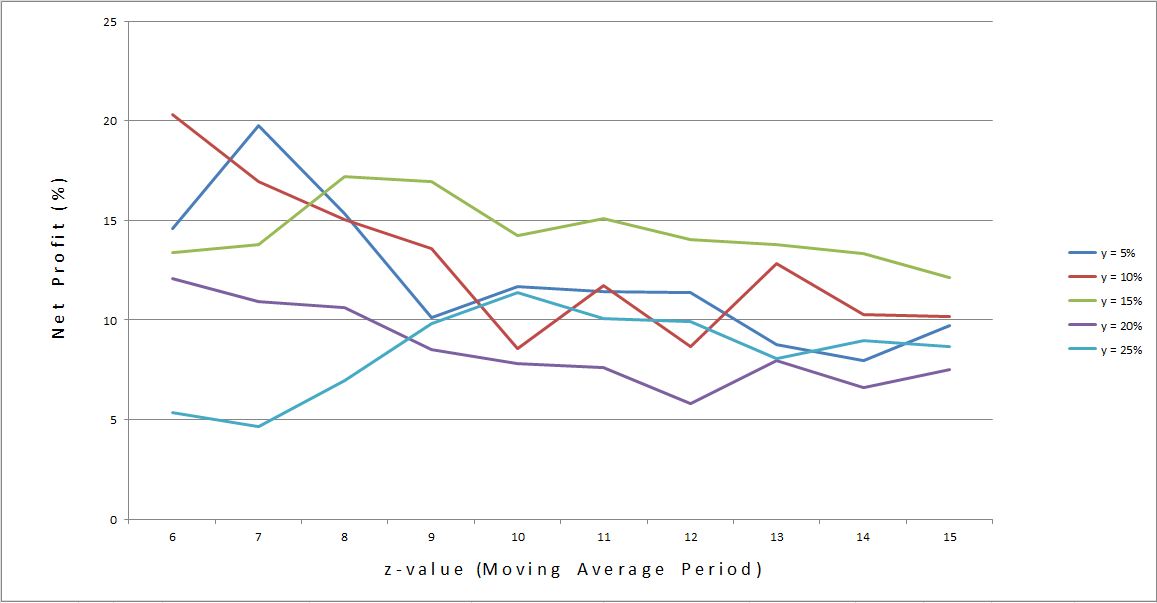
Following the course of evolutionary operation, I now want to analyze returns of each y-value individually:

What line(s) has large plateau regions rather than spike regions?  The red line seems to dive early (e.g. from z = 6-10) and then flatten out.  The blue line goes up and then way down before flattening.  The green line seems relatively flat.  The light blue line rises early on and then retraces half that rise.  The purple line falls gradually but seems pretty flat from z = 9-15.

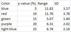
This eyeball method is consistent with a cursory statistical analysis:

Green and purple lines vary the least (flatness).

The one problem I have with this method is the percentage nature of the dependent variable.  That is, falling from 20(%) to 15(%) or 10(%) to 5(%) are both a range of 5% but the former is a 25% difference whereas the latter is a 50% difference.

That criticism aside, based on these data I would choose y = 15% and z = 10 (near the middle of plateau regions).

I will continue this analysis in future posts.

Trading System #1–SPY VIX (Part 3)

In http://www.optionfanatic.com/2012/10/01/trading-system-1-spy-vix-part-2/ (10/1/12), I continued the discussion of evolutionary operation by reviewing optimization.  Today I will begin the optimization process for the trading system.

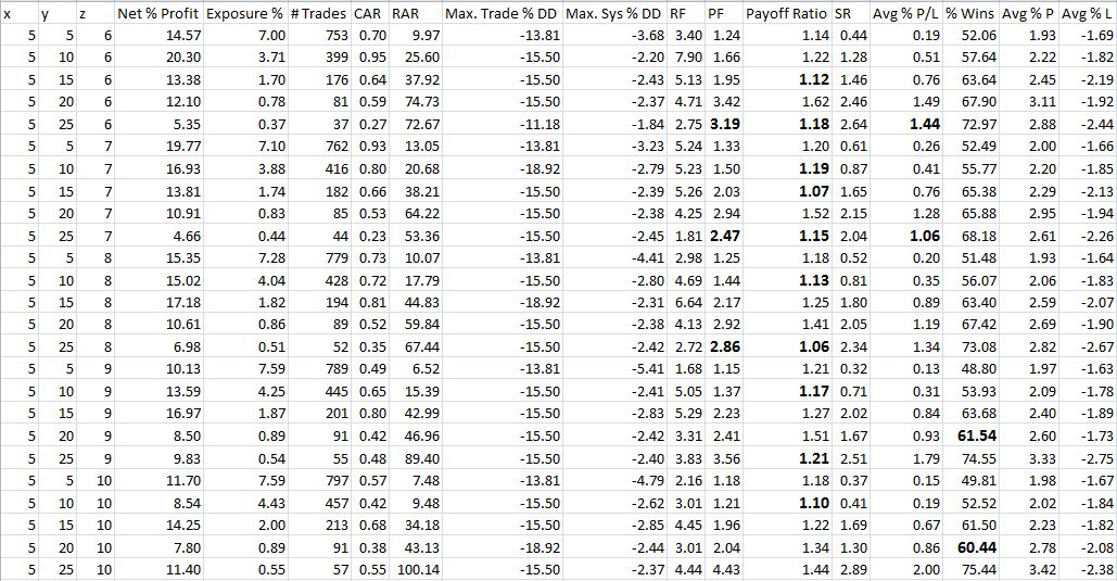
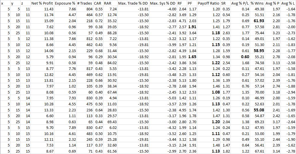
For the initial backtest, I am going to leave x fixed at 5 days and, as mentioned in the last blog post, vary y from 5-25 in increments of five [e.g. 5 (percent), 10, 15, 20, or 25] along with z from 6-15 in increments of one.  Other backtesting assumptions were discussed in “Trading System #1–Backtesting Assumptions” from 9/14/12.  The only change here is that I will take long and short SPY trades when VIX is “overbought” and “oversold,” respectively.

Table 2A

Table 2B

I abbreviated headings to make the Table font larger:

CAR = Compound Annualized Return (%)
RAR = Risk Adjusted Return (%) = CAR / Exposure %
Max. Trade % DD = Largest intratrade drawdown (%) (denominator is position size)
Max. Sys % DD = Largest portfolio drawdown (%) (denominator is current account value)
RF = Recovery Factor = Net profit / Max. System DD (higher is better)
PF = Profit Factor
Payoff Ratio = Average win / Average loss (second term of PF calculation)
SR = Sharpe Ratio
Avg % P / L = Average % gain or loss per trade
Avg % P = Average % profit on winning trades
Avg % L = Average % loss on losing trades

Several trends are evident from studying these results.  The numbers in bold and larger font are unexpected values with regard to these trends.  Feel free to take some time to peruse the Tables.

In my next post, I will begin the data dissection.

Trading System #1–Initial Assessment (Part 6)

In my post http://www.optionfanatic.com/2012/09/25/trading-system-1-initial-assessment-part-5/ (9/25/12), I finished up my analysis of the overbought VIX trading strategy.  Today I want to study the claim of avoiding SPY when VIX is oversold, which I described in http://www.optionfanatic.com/2012/09/13/trading-system-1-introduction/ (9/13/12).

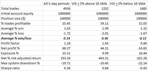
Do 5-day long trades in SPY actually lose money if placed when VIX is over 5% or more below its 10-SMA (“oversold”)?  I have included these results in the third column in order to compare with all 5-day SPY trades and 5-day SPY trades only when VIX is “overbought”:

Indeed, the oversold VIX strategy loses money.  Average % win is much smaller (1.32%) and the lower % trades profitable (52.05%) contributes to a negative profit factor and negative Sharpe ratio.

Now having substantiated both of the initial claims, I feel more confident about putting forth time and effort to try and develop a trading system.  I will continue with these steps in my next post.

Trading System #1–Initial Assessment (Part 5)

We have been studying the difference between 5-day long trades in SPY with daily entry vs. with entry only when VIX closes at least 5% above its 10-SMA (“overbought”).  Going back to Table 1 from my post http://www.optionfanatic.com/2012/09/19/trading-system-1-initial-assessment-part-1/ (9/19/12), today we will discuss the remaining results.

The overbought VIX strategy gets a slight edge with regard to % profitable:  59.11% to 55.45%.  In a broad sense, systems are usually trend-following or mean-reverting (i.e. sell when the market is strong and buy when the market is weak).  Trend-following systems typically have a lower % of profitable trades whereas mean-reverting systems have a higher % of profitable trades.  Trend-following systems typically have a much better average % win (for winning trades) to average % loss (for losing trades) ratio, however.  This is the tradeoff.  Recall that % profitable trades and average gain/loss are the two components of profit factor (PF) calculation.

The final statistic is the one I highlighted with bold:  average % win/loss.  In looking at Table 1, this statistic seemed to be the coup de grace for the “overbought” VIX strategy.  With both strategies having similar winning percentages, the “overbought” VIX strategy dominated with a 0.36% vs. 0.14% average % win/loss.  This difference is also reflected in the PF although the difference is not as clear (1.43/1.18 << 2).  The difference is reflected in the SR but as previously discussed SR is shroud in more complexity and controversy as a meaningful number.  One needs to have studied many systems before developing an intuitive understanding of how SR differences may reflect system performance.

In my post http://www.optionfanatic.com/2012/09/13/trading-system-1-introduction/ (9/13/12), I mentioned the internet claim that “when VIX closes 5% or more above its 10-SMA, SPX has outperformed the average week better than 2-1 over the next five trading days.”  Based especially on this average % win/loss statistic, I consider that claim to be verified.

This now leaves us to determine SPX (SPY) performance when VIX is “oversold.”  I will address this in the next post.