Investing in T-bills (Part 3)

In Part 2, I wrote about investing in T-bills while buying calls (also known as “long calls”) in the same account. Today, I will review that discussion and introduce put selling (also known as “short puts” or “naked puts”).

Long calls generally increase in value with the underlying stock once the increase is enough to offset the initial premium previously described as “rent.” In that example from the sixth paragraph here), I pay $13.73/share premium to buy the calls. After 62 days, my position will be profitable if SPY stock [an ETF] has gone up more than $13.73/share and no limit exists to how profitable these may be (net the initial $13.73 premium). If SPY increases less than $13.73/share, my position loses money. If SPY does not increase at all after 62 days, then my whole investment is lost (albeit only 2.7% of the cost to buy 200 shares outright).

I can only buy as many calls as the free cash in my account will allow (self-imposed guideline: I never want to borrow brokerage funds and owe upwards of 13% interest). Buying calls decreases free cash that may be used for T-bill investing.

Aside from buying calls, another way to participate in the movement of underlying stock is to sell puts. Long (bought) puts generally gain value as the underlying stock falls and sold (short) puts generally gain value as the underlying stock rallies. Selling puts allows me to collect premium rather than paying it; this provides a margin of safety if the underlying stock falls.

As an example, rather than buying the calls previously discussed, suppose I collect the $13.73/share premium by selling the corresponding puts.

The story is now different in several ways:

• First, the premium received for put sales (vs. premium due for call purchase) increases the cash balance in my account that I can use to buy T-bills.
• Second, if SPY increases over 62 days, then I keep the $13.73/share profit (vs. having to overcome any premium paid for profitability).
• Third, $13.73/share is my maximum potential profit (vs. unlimited profit potential net premium paid for long calls).
• Fourth, if SPY decreases up to $13.73/share, then I will have to surrender up to the entire premium received after 62 days. A net loss results if SPY decreases more than $13.73 (vs. long calls that incur maximum loss if SPY goes down at all). Potential loss on the short put is nearly unlimited except for the $13.73/share premium initially received.

I will continue next time.

Investing in T-bills (Part 2)

Last time I presented Investopedia information on the basics of T-bills: what they are, how they work, etc. Today I’m going to start discussing why to consider investing in them.

I invest in T-bills to get a better interest rate on cash than I otherwise would. I tend to have free cash in my brokerage account. The brokerage currently pays 0.35% interest on that cash. According to the Bankrate website, the national average yield for savings accounts is 0.57%. T-bills are currently paying over 5.0% interest.

Borrowing brokerage money to invest in T-bills would be a losing proposition. Suppose I open a margin account with $100,000 cash. I can buy stock with $100,000 and T-bills with $50,000. I will make 5% interest on the T-bills, but since that $50,000 is borrowed from the brokerage I will have to pay upwards of 13% interest. This is a guaranteed loss of at least (13% – 5%) = 8%. Bad idea… really bad idea.

For those investing in stocks, T-bills may not add much benefit. A stock investor opens a brokerage account to buy stocks. Most of the cash will therefore be deployed to that end. $95,000 may be used to purchase stock in a $100,000 account. This leaves only $5,000 to buy T-bills. It may still be worthwhile to do so, but T-bill investing does carry a minimal time commitment (to be discussed later).

Because options are leveraged instruments, cash outlays are different. Options allow me to control stock for a fraction of the cost. This means more leftover cash that I can conceivably use to purchase T-bills.

Imagine buying calls in the hypothetical account discussed above. With SPY at $509.83/share, I can buy 200 shares of SPY for $101,966. Alternatively, two 510 calls would cost me $2,746. This allows me to effectively rent 200 shares of SPY for 62 days. My position is then worth the difference of SPY and $510 [multiplied by two (options)]. If SPY is less than $510 then my position expires (i.e. “goes out,” “ends up”) worthless. If SPY is at $524, then my position is ~$2,800 (slight gain). If SPY is at $530, then my position is ~$4,000 [a much larger (percentage) gain].

With calls, I take on the risk of losing the full $2,746, but this is only 2.7% of the cost to buy shares. The leftover cash can be used to purchase T-bills. Interest received would be 0.05 * (100,000 – 2,746) * (62 / 365) ~ $849. With shares, because I borrowed $1,966 to establish the full position, I would actually owe 0.13 * 1,966 * (62 / 365 ) ~ $43 . The difference is $892 in about two months.

Interest aside, at the end of those two months the SPY position could also be down $2,746 were SPY to fall $13.73 (to $496.10/share). While this is an equivalent loss to the option position, I retain ownership of the shares and can subsequently recoup the loss if SPY moves higher. Expiring worthless means the option position can never rebound.

I will continue next time.

Investing in T-bills (Part 1)

I find an advantage to investing in Treasury Bills, but I am still trying to wrap my brain around how big a benefit this is, to what extent it may be utilized, and/or how much of it is real or just perceived.

Here are some basics courtesy of Investopedia:

     > A Treasury bill [T-bill]… is a short-term U.S. government debt obligation
     > backed by the Treasury Department with a maturity of one year or less.
     > T-bills are usually sold in denominations of $1,000… These securities are
     > widely regarded as low-risk and secure investments.
     >
     > The U.S. government issues T-bills to fund various public projects, such
     > as the construction of schools and highways. When an investor purchases
     > a T-bill, the U.S. government effectively writes an IOU to the investor.
     > Thus, T-bills are considered a safe and conservative investment since the
     > U.S. government backs them.
     >
     > T-bills are generally held until the maturity date. However, some holders
     > may wish to cash out before maturity and realize the short-term interest
     > gains by reselling the investment in the secondary market.
     >
     > T-bills can have maturities of just a few days, but the maturities listed by
     > the Treasury are are four, eight, 13, 17, 26, and 52 weeks.
     >
     > T-bills are issued at a discount from the par value (also known as the face
     > value) of the bill, meaning the purchase price is less than the face value of
     > the bill. So, for example, a $1,000 bill might cost the investor $950.
     >
     > When the bill matures, the investor is paid the face value—par value—of
     > the bill they bought. If the face value amount exceeds the purchase price,
     > the difference is the interest earned for the investor.
     >
     > T-bills do not pay regular interest payments as with a coupon bond, but a
     > T-bill does include interest, reflected in the amount it pays when it matures.
     >
     > The interest income from T-bills is exempt from state and local income
     > taxes. However, the interest income is subject to federal income tax.
     >
     > New issues of T-bills can be purchased at auctions held by the
     > government on the TreasuryDirect site. These are priced through a
     > bidding process, with bidders ranging from individual investors to
     > hedge funds, banks, and primary dealers. These purchasers may then
     > sell the bills to other customers in the secondary market…
     >
     > You can also buy Treasury bills through a bank or a licensed broker
     > [i.e. secondary market]. Once completed, the purchase of the T-bill
     > serves as a statement from the government that says you are owed
     > the money you invested, according to the terms of the bid.

I will get more into the details of investing with T-bills next time.

Time Spread Backtesting Concepts (Part 3)

Today I conclude this brief mini-series detailing background concepts about time spreads.

Theta is one parameter I found insidious in manual backtesting. 2020-2021 time spreads generally have a lot of “jump.” They seem to hit profit targets quickly and sometimes completely out of the blue (e.g. with PnL small or negative just a day or two beforehand). 2017 time spreads, in contrast, move very slowly. Weeks go by without any significant profit and loss is more common. Perhaps because I monitored the TD ratio per guidelines shown here, I did not think to track theta itself.

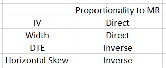
2017 volatility is extremely low and I eventually realized that position theta is extremely low with these guidelines, too. Over a given period, the market can be expected to move within a probability cone. When theta is much lower, profit will not accumulate to offset this movement. Without normalizing theta by adjusting spread width, these guidelines really describe entirely different strategies for 2017 and 2020/2021. As shown in the table here, width will affect MR, which can then be normalized as discussed in that final paragraph.

Eventually, I would like to do a study with no profit targets or stop-losses. Track MFE with DTE, MAE with DTE, and then visualize to check for optimal values. This should be done in walk-forward fashion to avoid generalized curve-fitting. Maybe every month I visualize a chart of MAE/MFE over the previous six months to see what values are optimal based on recent history. These values may or may not be stable going forward.

To get started, something simpler like backtesting with a straight 10% profit target and -20% max loss could be done. I should then try to generate a variety of combinations to verify the strategy as profitable in all cases. Other pairs could be 10%/-10%, 15%/-20%, 20%/-20%, 20%/-15%, etc. Of course, the higher the number the longer the trades. For this reason, some measure of PnL%/day also makes sense…

…and by now I have lost the “simpler” part. Keeping complexity out is certainly one of the larger challenges here.

Rewind: start with +10%/-20%. I can then compare strike selection from -5% to ATM to +5% by increments of 1%, 2%, or 2.5% to assess directional bias. Transaction fees should be included, and avoiding less-liquid strikes is a possibility.

As one last piece of theoretical complexity, I suspect an X% change in horizontal skew has less effect on PnL as DTE decreases. Lower DTE means less extrinsic value remains in the short option to be affected by IV change in the first place. Tracking horizontal skew % may therefore be misleading unless done with regard to DTE.

Time Spread Backtesting Concepts (Part 2)

Today I want to continue with background on time spreads before moving forward with Python backtesting.

How horizontal skew reacts to different types of market rallies and/or selloffs is hard to predict. In selloffs when fear spikes, traders tend to buy near-term options pressuring term structure toward backwardation (increasing horizontal skew). In theory, increased IV is good for vega-positive time spreads. If horizontal skew becomes more positive, then although the long leg increases in value (good) due to IV, short-leg value may increase more (bad). The overall effect on PnL depends on how decreased spread value from higher skew compares with increased spread value from higher long option prices.

You can imagine other permutations for cases where horizontal skew is initially positive or negative, becomes more positive or negative based on different magnitudes of rally/selloff, etc. I am interested to see if any significant association exists between [changes in] horizontal skew and profitability.

I am also interested to see if any significant association exists between IV and profitability. Conventional wisdom says vega-positive time spreads should be purchased when IV is low. Could horizontal skew have a significant interaction here?

Margin requirement (MR) varies from one time spread to another and I have had difficulty putting my finger on this. MR is proportional to IV. MR should be inversely proportional to DTE since all else being equal, time spread price increases over time and maximum potential risk is the cost. Width (days between expirations) is directly proportional to MR because for the same short option, long options farther out in time are more expensive. Horizontal skew should also be inversely proportional to MR because the higher skew means a more-expensive near-term option and lower overall cost.

To simplify things a bit:

Perhaps Python can aid with some analysis here.

With MR so variable, some consideration must be given to position sizing. One possibility is a fixed position size backtest where each trade is done with number of contracts (rounded down) equal to position size ($) / MR. Alternatively, a fixed percentage of the total account could be allocated. This would allow for compounding. Drawdowns across the equity curve could then be compared as percentages off the highwater mark to normalize for temporal sequence. This seems logical at first glance.

I will continue next time.

Practice Trades Cal 1.13

Cal 1.13 (guidelines here) begins 2/18/20 (87 DTE) with SPX 3370 and trade -$168 (-2.6%). TD = 1, MR $6,498 (two contracts), IV 11.9%, horizontal skew -0.85%, NPD 6.8, and NPV 231.

What jumps out at you when looking at the initial risk graph?

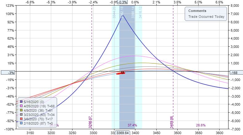
This is the second Cal example where the same strike is unavailable in the back month (see Cal 1.4 here). Placing the long leg lower gives the trade a bullish bias, which is something discussed in the fifth paragraph here.

Notice that a bullish bias is achieved whether I diagonalize the long leg (lower) or whether I raise the calendar strike. The former preserves profit potential at current underlying price at the cost of raising MR. Each has pros and cons.

As mentioned in the third paragraph here, I may want to come up with some alternative downside management since TD = 1 at inception unless I plan to let it go to ML.

On 84 DTE, trade -4.4% with market down 0.85 SD in three days.

Exit 81 DTE for loss of $1,478 (-22.8%). This is the 4.33 SD down day, which comes without warning. Over 6 days, SPX down 2.73 SD with IV up 83%. Horizontal skew has increased slightly to -0.62%. TD = 0 (rounded).

Unlike Cal 1.2, SOH to see how the market “shakes out” would be a terrible decision here:

Highlighted is my first opportunity to exit at max loss (with market far outside profit tent and TD 0 unlike third paragraph here where Cal 1.12 is still well-positioned with TD strong). I have to take the loss immediately: no reason not to.

HEED WARNING DISCRETIONARY TRADERS!

I think one of the biggest risks of discretionary trading is the tendency to see something that seems to work while conveniently forgetting other instances where it does not. You may be confident in something that, on the whole, adds no benefit (or worse). A large-sample-sized systematic backtest to assess strategy guidelines can prevent this from happening.

Practice Trades Cal 1.12 (Part 2)

I left off questioning whether I should exit Cal 1.12 at max loss despite being well-positioned inside the profit tent.

From a systematic, programming standpoint, I don’t see how to do breakeven (BE) estimation with time spreads without Black-Scholes and/or volatility skew modeling. This precludes implementation of a Python backtester.

From an “art of trading” standpoint, my gut says “no way no how” do I take max loss when I am well inside the profit tent (strongly supportive of a high TD) like this.* To convince me otherwise, I will be on the lookout for cases where I remain in such trades only to meet a horrific demise.

Exit two trading days later at 73 DTE for profit of $552 (15.3%). SPX is up 0.13 SD to 3011 with IV up 5.9% over the 5 days, TD = 96, and horizontal skew remaining at +1.8%.

Part of me wonders if it might require extraordinary discipline to exit still being positioned near the center with TD so high.

If I stayed in, then when would I look to exit?

Moving ahead to 11 DTE:

I am now approaching the downside BE. While still 140 points away, I am certainly getting to the “slim pickins'” portion of the graph compared to what lies to the right. TD is 10 at this point and trade is +42.5%, which would be an absurd amount to lose should the market continue lower.

This would be a decent time to exit. I may not be able to code this discretionary interpretation, but said “art of trading” still seems alluring as a viable tool.

Finally, I’m a bit curious about the margin requirement (MR). I mentioned in this third paragraph that high IV may cause time spreads to be expensive. Such is not the case with Cal 1.12. I will grant that Cal 1.12 IV (~35%) is nowhere near that seen in Cal 1.3, but it still seems relatively high whereas MR seems relatively low. With starting DTE, horizontal skew, and [average] IV [proprietarily calculated over the whole option matrix in ONE] all potential contributing factors, how can this be explained?

I will pick up here next time.

* — This is 31.3% of the way between BEs.

Practice Trades Cal 1.12 (Part 1)

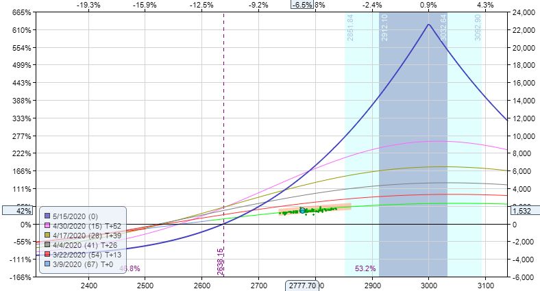
Cal 1.12 (guidelines here) begins 2/27/20 (78 DTE) with SPX 2995 and trade -$168 (-4.3%). MR is $3,608 (two contracts), TD 53, IV 35.2%, horizontal skew +1.8%, NPD 0.8, and NPV 224.

“Conventional wisdom” (see second paragraph) would probably suggest skipping this day for entry given a crazy market down 3.1 SD! I can imagine a volatile, whipsaw market causing hefty slippage, but looked at another way if I place a limit order and just wait, then I can imagine having a good chance to be filled precisely because of the market’s wild movement.

The positive horizontal skew provides me with a little extra bonus compensation for the risk taken in a volatile market.

How much compensation, you ask?

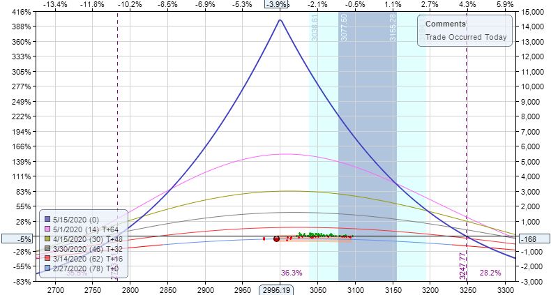
I admittedly zoomed in to make this look super large. However, what is no joke is 460 points between expiration breakevens (BE)—a full 15% of the underlying’s current price. If volatility tanks then the graph will move down and BEs will narrow, but as the positive skew reverts, T+0 will rise. Lots of moving parts here.

Surprisingly [to me], the official max loss (-$728, -20.2%) is hit the very next day with market down 1.1 SD:

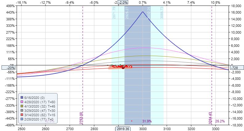
Should I exit this trade?

The market is down 59 points, but I still have 166 points to downside BE. Distance between expiration BEs has increased to 530 points with IV now at 45.4%. Horizontal skew has increased and I still expect a reversion to negative horizontal skew to follow (recall last paragraph here). TD 25 also suggests solid potential for profit potential going forward.

I will continue next time.

Practice Trades Cal 1.11A

Look back at the previous two practice trades (guidelines here unless otherwise stated). Both start out with negative skew, but Cal 1.10A requires a bullish bias (-0.65 delta) to profit. To be fair, I should also look at Cal 1.11 with a bullish bias.

Cal 1.11A begins 5/11/20 (67 DTE) with SPX 2934 and 3060 puts -$168 (-2.6%). MR is $6,418 (two contracts), TD 2, IV 22.0%, horizontal skew -0.2%, NPD 8.8, and NPV 262.

With TD starting at 2, a different management plan may be advised as trade begins very close to an adjustment point. ML may also need tweaking since it can arrive sooner with directional bias. I haven’t been monitoring data on this (and don’t intend to), but the ONE model currently shows T+0 100 points above downside ML and only 20 points from downside expiration breakeven (BE). I would guess these numbers to be less than a NTM time spread with TD starting much higher.

Whatever management thresholds I choose, no right answer(s) may exist because any will have its pros and cons. Even more difficult is determining something consistent between historical backtesting and future live trades.

Getting back to the current Cal 1.11A, MDD is -$1,188 (-18.5%) on 2 DIT: just a stone’s throw away from ML. This is a case in point, although the quick loss does come on the heels of back-to-back 1+ SD down days: a rarity.

Exit trade 52 DTE for profit of $802 (12.5%). SPX up 0.42 SD with IV up 5.9% over the 15 days. Horizontal skew has decreased to -1.2%, which is not good for getting into the trade but can be very good while in the trade. TD = 5 at PT.

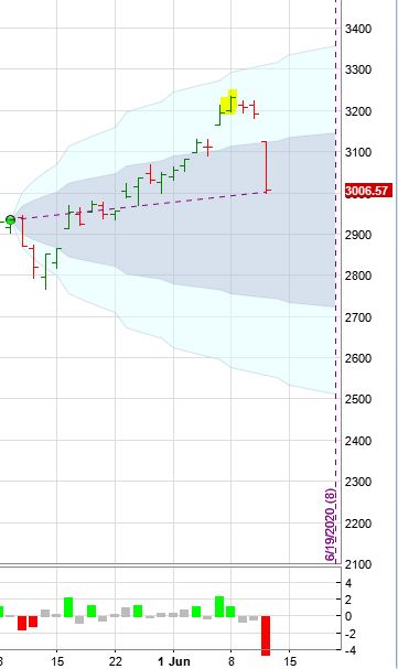
A study of MFE would be interesting to determine whether any sort of PT is optimal. 1.11A goes on to gain $1,662 (25.9%) at 43 DTE before slipping back to +$642 (10%) with TD 5 the next trading day after that. PnL dips the next trading day (39 DTE) to 7.7% (TD 5) before soaring to +45.7% three trading days later at 36 DTE on a 4.6 SD downmove (see price chart here).

I would be interested to collect MFE data in a Python program (as mentioned in the third paragraph here).

Bottom line for today: like Cal 1.10, a bullish bias in this negatively skewed Cal 1.11 ends up profitable as well.

Practice Trades Cal 1.10 – 1.11

Cal 1.10 (guidelines here) begins 5/4/20 (74 DTE) with SPX 2838 and 2840 puts -$168 (-2.4%). MR is $7,128 (two contracts), TD 29, IV 31.4%, horizontal skew -0.02%, NPD 1.4, and NPV 216.

MDD is -$1,048 (-14.7%) on 44 DTE.

Exit trade 42 DTE for loss of $2,158 (-30.3%). SPX up 1.3 SD to 3190 with IV down 40% over the 32 days. Horizontal skew up to +0.6%. This trade exits on that same big up day as Cal 1.9 with a 2.2 SD one-day rally.

Anecdotally speaking (since I’ve only backtraded 10 so far), the last two calendars have not had the snap seen in some earlier ones. With the high IV “juice” and/or [significant] positive skew, perhaps it’s not unusual for calendars to reach PT in sudden, unexpected fashion. In contrast, this trade (and the second half of Cal 1.9) faces a market steadily grinding higher.

What if I placed Cal 1.10 at -0.65 delta rather than the first 10-point strike above the money?

Cal 1.10A begins 5/4/20 (74 DTE) with SPX 2838 and 3000 puts (roughly -0.65 delta) -$168 (-2.4%). MR is $6,578 (two contracts), TD 3 (expectedly lower being farther ITM), IV 31.4%, horizontal skew -0.6%, NPD 7.7, and NPV 241.

MDD is -$448 (-6.8%) on 65 DTE.

Exit trade 56 DTE for profit of $742 (11.3%). SPX up 0.58 SD with IV down 24% over the 18 days. Horizontal skew has decreased to -1.0%, which is not good for getting into the trade but can be very good while in the trade.

In this instance, leaning bullish rewrites history. Whether this accurately reflects a larger sample size remains to be seen.

Cal 1.11 begins 5/11/20 (67 DTE) with SPX 2934 and 2940 puts -$168 (-2.4%). MR is $7,128 (two contracts), TD 19, IV 22.0%, horizontal skew -0.9%, NPD 1.6, and NPV 233.

MDD is -$1,378 (-19.3%) on 39 DTE: just a slight breeze shy of ML.

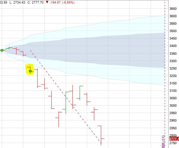
Exit trade 36 DTE for profit of $2,282 (32.0%). SPX up 0.38 SD with IV up 80% over the 31 days. Horizontal skew has increased to +1.3%. The underlying price action behind this trade is as follows:

The gradual, grinding-higher market resulted in two consecutive losers. This is almost the third. MDD occurs on the highlighted bar, which is just three days before a 4+ SD downmove carries home the W. The highlighted bar presses the market well into the second SD of the probability cone: an extreme I suspect usually does not persist [but most certainly can].

Trading’s version of Bruce Willis (apologies in advance) is mean reversion with a vengeance.